How we almost hacked the Phobos ransomware using CUDA

For the past two years, we have been working on a proof-of-concept decryptor for the Phobos ransomware family. For reasons we will explain here, it is impractical. So far, we haven’t been able to use it to help a real victim. But we decided to publish the results and tools in the hope that someone will find them useful, interesting, or continue research.

We describe the vulnerability and how we reduced the computational complexity and increased the performance of the decryptor to achieve an almost practical implementation. Continuation – to the start of our course “White hacker”

What where When

Phobos is the inner and largest natural satellite of Mars. It is also the name of a widespread ransomware family, Phobos, which was first seen in early 2019. The program is not very interesting – it has a lot in common with the “Dharma” and is probably written by the same authors.

We started the study after several important Polish organizations were encrypted with the Phobos ransomware in a short time. It became clear that Phobos’ key scheduling feature was unusual; you can even say that it is broken. This prompted further research in the hope of creating a decoder.

Reverse engineering

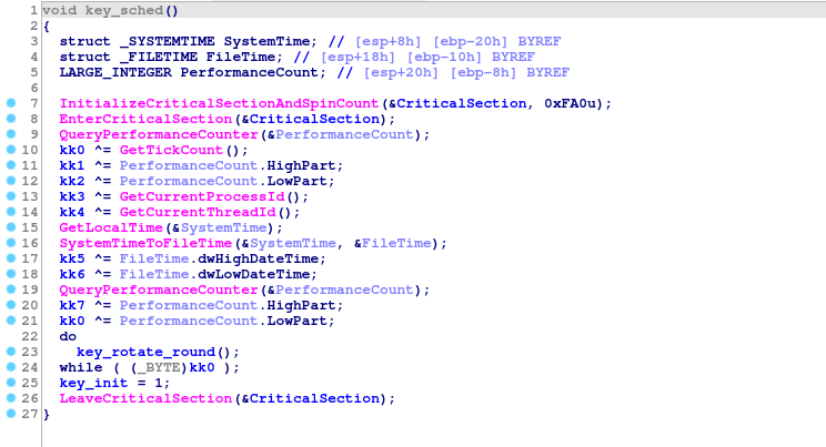
Let’s skip the boring details: debugging protection features, deleting shadow copies, bypassing the main disk, etc. The most interesting feature for us is the key scheduling:

It is curious that instead of one good source of entropy, the author of the malware decided to use several bad ones. The list contains:

• Two calls to the QueryPerformanceCounter() function.
• GetLocalTime() + SystemTimeToFileTime().
• GetTickCount().
• GetCurrentProcessId().
• GetCurrentThreadId().

Finally, a variable but deterministic number of SHA-256 rounds is applied. On average, it takes 256 SHA-256 executions and one AES decryption to verify a key.

It immediately sounded alarm bells in our heads. Assuming that the infection time is known to within 1 second (for example, through the timestamps of files or logs), it turns out that the number of operations required to enumerate each component is:

Operation Number of operations

QueryPerformanceCounter 1 10**7

QueryPerformanceCounter 2 10**7

GetTickCount 10**3

SystemTimeToFileTime 10**5

GetCurrentProcessId 2**30

GetCurrentThreadId 2**30

Obviously, each component can be brute-forced independently, because 10**7 is not so much for modern computers. But is it possible to recover the whole key?

How many keys do we actually need to check?

Initial state (141 bits of entropy)

The number of keys for a naive brute-force attack is:

>>> 10**7 * 10**7 * 10**3 * 10**5 * 2**30 * 2**30 * 256
2951479051793528258560000000000000000000000
>>> log(10**7 * 10**7 * 10**3 * 10**5 * 2**30 * 2**30 * 256, 2)
141.08241808752197  # that's a 141-bit number

A huge, incomprehensibly large number. Not the slightest chance of brute force.

But we are not the type to give up easily.

Can I get your PID? (81 bits of entropy)

Let’s start with some assumptions. We have already done one thing: thanks to the system/file logs, we know the time with an accuracy of 1 second. One source of such data can be the Windows event logs:

There is no default event that fires for each new process, but with sufficient attention to analysis, it is often possible to recover the PID and TID of the ransomware process.

Even if it is not possible to set them, because Windows PIDs are consistent, it is almost always possible to limit them by a significant amount. This way, we usually don’t have to iterate over the entire space in 2**30.

Let’s assume that we already know the PID and TID (main thread) of the ransomware process. Don’t worry, this is the biggest assumption in this entire article. Will this make things easier for us?

>>> log(10**7 * 10**7 * 10**3 * 10**5 * 256, 2)
81.08241808752197

81 bits of entropy is too much to think about brute force, but we have achieved something.

Δt = t1 – t0 (67 bits of entropy)

Here’s another reasonable guess: two consecutive calls to QueryPerformanceCounter will return similar results. In particular, the second QueryPerformanceCounter will always be slightly larger than the first. There is no need to iterate over both counters – we can iterate over the first one and then guess the time between executions.

If we take the code as an example, instead of

for qpc1 in range(10**7):
    for qpc2 in range(10**7):
        check(qpc1, qpc2)

you can write:

for qpc1 in range(10**7):
    for qpc_delta in range(10**3):
        check(qpc1, qpc1 + qpc_delta)

The number 10**3 is empirically determined to be sufficient. In most cases, this should be enough, although it is only 1ms, so in case of a very bad context switch, it will fail. Let’s try anyway:

>>> log(10**7 * 10**3 * 10**3 * 10**5 * 256, 2)
67.79470570797253

In any case, who needs the exact time? (61 bits of entropy)

2**67 calls to sha256 is a lot, but the number becomes manageable: by coincidence, it almost exactly matches the current BTC hashrate. If instead of burning electricity senselessly, the entire BTC network was repurposed to decrypt Phobos victims, then that network would decrypt one victim per second, assuming the PID and TID are known.

So SystemTimeToFileTime can have 10ms precision. But GetLocalTime is not:

This means that only 10**3 options need to be iterated over, not 10**5:

>>> log(10**7 * 10**3 * 10**3 * 10**3 * 256, 2)
61.150849518197795

Mathematical time (51 bits of entropy)

Maybe it will be possible to find a better algorithm? There are no more obvious things to optimize.

Please note that key[0] equals GetTickCount() \^ QueryPerformanceCounter().Low. A naive iteration algorithm will test all possible values ​​of both components, but in most cases much more can be achieved. For example, 4 ^ 0 == 5 ^ 1 == 6 ^ 2 = ... == 4. We only care about the end result, so the timer values, which end up being the same key, can be ignored.

An easy way to do this looks like this:

def ranges(fst, snd):
    s0, s1 = fst
    e0, e1 = snd
    out = set()
    for i in range(s0, s1 + 1):
        for j in range(e0, e1 + 1):
            out.add(i ^ j)
    return out

Unfortunately, this is quite CPU intensive (we want to squeeze as much performance as possible). It turns out there is a better recursive algorithm. It allows you not to waste time on duplicates, but is rather subtle and not very elegant:

uint64_t fillr(uint64_t x) {
    uint64_t r = x;
    while (x) {
        r = x - 1;
        x &= r;
    }
    return r;
}

uint64_t sigma(uint64_t a, uint64_t b) {
    return a | b | fillr(a & b);
}

void merge_xors(
    uint64_t s0, uint64_t e0, uint64_t s1, uint64_t e1,
    int64_t bit, uint64_t prefix, std::vector<uint32_t> *out
) {
    if (bit < 0) {
        out->push_back(prefix);
        return;
    }

    uint64_t mask = 1ULL << bit;
    uint64_t o = mask - 1ULL;

    bool t0 = (s0 & mask) != (e0 & mask);
    bool t1 = (s1 & mask) != (e1 & mask);

    bool b0 = (s0 & mask) ? 1 : 0;
    bool b1 = (s1 & mask) ? 1 : 0;

    s0 &= o;
    e0 &= o;
    s1 &= o;
    e1 &= o;

    if (t0) {
        if (t1) {
            uint64_t mx_ac = sigma(s0 ^ o, s1 ^ o);
            uint64_t mx_bd = sigma(e0, e1);
            uint64_t mx_da = sigma(e1, s0 ^ o);
            uint64_t mx_bc = sigma(e0, s1 ^ o);

            for (uint64_t i = 0; i < std::max(mx_ac, mx_bd) + 1; i++) {
                out->push_back((prefix << (bit+1)) + i);
            }

            for (uint64_t i = (1UL << bit) + std::min(mx_da^o, mx_bc^o); i < (2UL << bit); i++) {
                out->push_back((prefix << (bit+1)) + i);
            }
        } else {
            merge_xors(s0, mask - 1, s1, e1, bit-1, (prefix << 1) ^ b1, out);
            merge_xors(0, e0, s1, e1, bit-1, (prefix << 1) ^ b1 ^ 1, out);
        }
    } else {
        if (t1) {
            merge_xors(s0, e0, s1, mask - 1, bit-1, (prefix << 1) ^ b0, out);
            merge_xors(s0, e0, 0, e1, bit-1, (prefix << 1) ^ b0 ^ 1, out);
        } else {
            merge_xors(s0, e0, s1, e1, bit-1, (prefix << 1) ^ b0 ^ b1, out);
        }
    }
}

Perhaps there is an algorithm simpler or faster, but the authors did not know about it when working on the decoder.

Here is the entropy after this change:

>>> log(10**7 * 10**3 * 10**3 * 256, 2)
51.18506523353571

This was the final difficulty reduction. What is missing here is a good implementation.

Speed

Naive implementation in Python (500 keys per second)

The original PoC in Python tested 500 keys per second. It takes 2314 processor days to enumerate 10**11 keys. This is far from practical. But Python is, in fact, the slowest in terms of high performance computing. More can be achieved.

Usually in situations like this we would implement our own decoder (in C++ or Rust). But even this is not enough here.

Time does wonders

We decided to achieve maximum performance and implement our solver in CUDA.

CUDA first steps (19166 keys per minute)

Our first naive version was able to crack 19166 keys per minute. We had no experience with CUDA, we made a lot of mistakes; GPU usage statistics looked like this:

sha256 improvement (50000 keys per minute)

Obviously, sha256 turned out to be a huge bottleneck: there are 256 times more calls to sha256 than AES. Much of the work here is focused on simplifying and adapting the code.

For example, we have built in sha256_update:

Built in sha256_init:

Replaced global arrays with local variables:

Hardcoded data size to 32 bytes:

And made a few operations more GPU-friendly, such as using __byte_perm for bswap.

In the end, the main loop has changed:

After this optimization, we realized that the code now makes a lot of unnecessary copies and data transfers. Now copies are not needed:

All this allowed us to increase productivity by 2.5 times – up to 50 thousand keys per minute.

Let’s parallelize the algorithm (105000 keys per minute)

Work is divided into threads, and the threads perform logical operations. In particular, memcopy to and from the graphics card can run concurrently with our code without any performance loss.

By simply changing our code to use threads more efficiently, we were able to double the performance to 105k keys per minute:

And finally AES (818000 keys per minute)

Despite all these changes, we didn’t even try to optimize AES. After all the lessons learned, it was pretty easy. We just looked for patterns that didn’t work well on the GPU and made the code better. For example:

We changed the naive for loop to a hand-rolled version that worked with 32-bit integers.

It may seem like a small thing, but in fact, the throughput has become significantly higher:

…and now in parallel (100 billion keys per minute)

We had the last trick in reserve – to run the same code on multiple GPUs! Conveniently, we have a small GPU cluster on CERT.PL. We provisioned two machines with a total of 12 Nvidia GPUs. Throughput immediately increased to almost 10 million keys per minute.

Thus, enumeration of 10**11 keys in a cluster takes only 10,187 seconds (2.82 hours). Sounds tempting, right?

Where did it all go wrong?

Unfortunately, as we mentioned at the beginning, there are many practical problems that we have briefly covered, this even made publishing the decryptor more difficult:

• Knowledge of TID and PID parameters is required. This makes it difficult to automate the decoder.
• We assume very accurate measurements of time. Unfortunately, such a measurement is complicated by clock drift and noise deliberately introduced into the Windows performance counters.
• Not every version of Phobos is vulnerable. Before deploying an expensive decoder, reverse engineering is required to confirm the family.
• Even after all the improvements, the code is too slow to run on a consumer-grade computer.
• Victims don’t want to wait for investigators with no guarantee of success.

That’s why we decided to publish this article and the source code of the (almost working) decryptor. Hopefully, this will give malware researchers a fresh look at the topic and perhaps even decipher ransomware victims.

We published CUDA source code. It contains a brief instruction, an example configuration and a set of data to test the program.

Ransomware sample analyzed: 2704e269fb5cf9a02070a0ea07d82dc9d87f2cb95e60cb71d6c6d38b01869f66 | MWDB | VT

Useful theory and interesting practice in our courses: