Classification of exoplanets (part II – building models)

This is the second and final part of the article, in which we consider the problem of classifying exoplanets. If the previous article was more about data preprocessing, then here we will build models, select the best and experiment.

PS some points may not be clear, so it’s better to start from the first part: https://habr.com/ru/articles/800999/

So, I hope that everyone who wanted to watched the first part, so we can start.

Random Forest

That time we selected features using the Gain method using a random forest, now let’s see how effective this was by building another random forest model.

rfi = RandomForestClassifier(max_depth=2, random_state=42)
rfi.fit(X_train[['koi_fpflag_nt', 'koi_fpflag_ss', 'koi_fpflag_co', 'koi_fpflag_ec',
       'koi_depth', 'koi_prad', 'koi_prad_err1', 'koi_prad_err2', 'koi_teq',
       'koi_insol_err1', 'koi_insol_err2', 'koi_model_snr', 'koi_steff_err1',
       'koi_steff_err2']], y_train)
rfi_pred_train=rfi.predict(X_train[['koi_fpflag_nt', 'koi_fpflag_ss', 'koi_fpflag_co', 'koi_fpflag_ec',
       'koi_depth', 'koi_prad', 'koi_prad_err1', 'koi_prad_err2', 'koi_teq',
       'koi_insol_err1', 'koi_insol_err2', 'koi_model_snr', 'koi_steff_err1',
       'koi_steff_err2']])
rfi_pred_test=rfi.predict(X_test[['koi_fpflag_nt', 'koi_fpflag_ss', 'koi_fpflag_co', 'koi_fpflag_ec',
       'koi_depth', 'koi_prad', 'koi_prad_err1', 'koi_prad_err2', 'koi_teq',
       'koi_insol_err1', 'koi_insol_err2', 'koi_model_snr', 'koi_steff_err1',
       'koi_steff_err2']])

In fact, it’s not very colorful to carry around this list of features, but I’m a lazy person, I saw the output of the features in Feature Selection, copied it, added parentheses [квадратные] and forward.

Let's look at the metrics

metrics(y_test,rfi_pred_test)

accuracy: 0.9456351280710925
f1: 0.94831013916501
roc auc: 0.9462939057241274

What kind of function is this? A reader who didn’t move on to the first part and was too lazy may ask. I don't judge. This is the function and here it is:

def metrics(y_true,y_pred):
    acc=accuracy_score(y_true, y_pred)
    f1=f1_score(y_true, y_pred)
    roc_auc=roc_auc_score(y_true, y_pred)
    print(f'accuracy: {acc}\nf1: {f1}\nroc auc: {roc_auc} ')

Since we will be building more than a few models, having such a function makes our life easier, an engineering solution, one might say)

Now let’s remember that we also used the F-test to select features and got the following list: [‘koi_fpflag_nt’, ‘koi_fpflag_ss’, ‘koi_fpflag_co’, ‘koi_fpflag_ec’, ‘koi_depth’, ‘koi_teq’, ‘koi_steff_err1’, ‘koi_steff_err2’] from it we simply take the variable X_f, which was declared in the code of the first part

y_f=y
X_f_train, X_f_test, y_f_train, y_f_test = train_test_split(X_f, y_f, test_size=0.2, random_state=42)
model_f=RandomForestClassifier(max_depth=2, random_state=42)
model_f.fit(X_f_train, y_f_train)
f_pred=model_f.predict(X_f_test)
metrics(y_f_test, f_pred)

accuracy: 0.9790904338734971
f1: 0.9801192842942346
roc auc: 0.9798926657489797

So far, F-test is the best thing that has happened to this data, I really like these metrics, but we won’t stop there.

XGBoost

Before building the XGBoost model, let's run it through GridSearchCV, most likely this will happen relatively quickly. I'll just note that the more parameters you decide to run, the longer it will take.
GridSearchCV allows you to select the best parameters for training the model; in my opinion, this function works faster with XGBoost than with Catboost, as well as the training process in principle. Maybe I'm wrong, so if anyone has thoughts on this matter, I'd like to hear them.
Let's start the process:

from xgboost import XGBClassifier
from sklearn.model_selection import GridSearchCV
xgbmodel = XGBClassifier()
parameters = {'learning_rate': [0.03, 0.1],
              'max_depth': [2,3.5, 10],
              'colsample_bytree': [0.7, 0.5, 1],
              'n_estimators': [0,150,10]}

xgb_grid = GridSearchCV(xgbmodel,
                        parameters,
                        cv = 2,
                        n_jobs = 5,
                        verbose=True)

xgb_grid.fit(X,y)

print(xgb_grid.best_score_)
print(xgb_grid.best_params_)

The output is this:
Fitting 2 folds for each of 54 candidates, totaling 108 fits 0.9807611877875366 {'colsample_bytree': 1, 'learning_rate': 0.03, 'max_depth': 2, 'n_estimators': 150}

we write these parameters into our XGBoost model

xgb=XGBClassifier(n_estimators=150, learning_rate=0.1, max_depth=2, colsample_bytree=0.7 ,randomstate=0)
xgb.fit(X_f_train, y_f_train)
metrics(y_test, xgb.predict(X_f_test))

accuracy: 0.9822268687924726
f1: 0.9831516352824579
roc auc: 0.982836728555653

The metrics are better than those of random forest, and in all 3 of its variations.
You can throw Gain on top and reduce the sample, but as for me, 8 parameters and such metrics are a good ratio. If someone has the desire, I think it won’t be difficult to implement the Gain method by analogy with Random-Forest (again, the previous article).

And we are taking the next step

CatBoost

The selection of parameters can also be done through Catboost, besides, it has its own method for this, which also builds a cool graph, but you will have to wait, and we already have the XGBoost parameters and I think no one will mind if we integrate them into Catboost with minor changes:

from catboost import CatBoostClassifier
cat=CatBoostClassifier(n_estimators=150, learning_rate=0.1, max_depth=2,bootstrap_type="Bayesian", task_type="GPU")
cat.fit(X_f_train,y_f_train, verbose=False)
cat_pred=cat.predict(X_f_test)
metrics(y_test, cat_pred)

Metrics:
accuracy: 0.9822268687924726
f1: 0.9831516352824579
roc auc: 0.982836728555653

So, from the point of view of classical ML, we implemented the most popular models and, as expected, received the best metrics on gradient boosting models.

Neural network on tensorflow

Now let’s check the thesis stated in Part I that this problem can be solved through a neural network.

First, let's standardize the data relative to the normal distribution.

mean=X_train.mean(axis=0)
std=X_train.std(axis=0)
X_train-= mean
X_train/= std
X_test-= mean
X_test/= std
#запринтим что мы сделали
print('train mean',X_train.mean(axis=0)[:5]) 
print('test mean',X_test.mean(axis=0)[:5]) 
print('train std',X_train.std(axis=0)[:5])
print('train std',X_test.std(axis=0)[:5])

std – standard deviation
mean – average

By the way, std will be equal to 1 for everyone in print

A small retreat

To build the neural network we will use tensorflow, which after version 2.11 stopped supporting GPU training on Windows; you can read more on their website: https://www.tensorflow.org/install/pip?hl=ru#windows-native_1
To solve this problem you need to install python version 3.9 (I have 3.9.18), you don’t need to delete the current Python, but for version 3.9 you need to create a separate virtual environment, for example through miniconda, download CUDA and CUDNN if you have NVidia, I don’t know about alternatives , since Nvidia itself has it. All the fun with the installation is that you need to choose the right versions of all these extensions and the tensorflow library. This can really take a lot of time if you haven’t done anything like this before, so this guy from YouTube can also help, who got confused and did a detailed installation of all Cuda and Cudnn: https://www.youtube.com/watch?v=xTF_n1jp9n8
However, he didn’t seem to talk much about the creation of a new Venv (virtual environment), so for those who are looking for Google, help.
An alternative to all this is either training on a CPU, that is, on a regular processor, or google Colab, where you can choose what your environment will run on and use the service’s benefits. Their capacity should be sufficient for this task.
Training on the GPU is clearly faster than on the CPU; an increase of 1.5-2 times can be obtained for sure.

Let's end this retreat

Let's set the model parameters, and before that, check if the GPU is working

import tensorflow as tf 
physical_devices = tf.config.list_physical_devices('GPU')
print("Num GPUs:", len(physical_devices))
#output: 1  если gpu работает

model = tf.keras.Sequential([
    tf.keras.layers.Dense(32, activation='relu', input_shape=(X_train.shape[1],)),
    tf.keras.layers.Dense(16, activation='relu' ),
                    
    tf.keras.layers.Dense(1, activation='sigmoid')
])
model.summary()

# Model: "sequential"
# _________________________________________________________________
#  Layer (type)                Output Shape              Param #   
# =================================================================
#  dense (Dense)               (None, 32)                1376      
                                                                 
#  dense_1 (Dense)             (None, 16)                528       
                                                                 
#  dense_2 (Dense)             (None, 1)                 17        
                                                                 
# =================================================================
# Total params: 1,921
# Trainable params: 1,921
# Non-trainable params: 0
# _________________________________________________________________

We train and look at losses

model.compile(optimizer="adam", loss="binary_crossentropy")

history = model.fit(X_train, y_train, epochs=16, verbose=1)

# Визуализация процесса обучения
plt.plot(history.history['loss'])
plt.xlim(-0.5,20)
plt.title('Loss')
plt.xlabel('Epoch')
plt.ylabel('Loss')
plt.show()

Let's use the Datagenerator, borrowed from this wonderful author from YouTube: https://www.youtube.com/watch?v=PLlic60dgS4&list=PLkJJmZ1EJno4lRvtQjQrNNACpeMLOd-SD&index=7

It sets batch_size, so if you want to get the result faster, then simply increase it, for example, to 16, 32 or 48, etc. The quality of the model will drop, but it will be built faster.

import numpy as np
from tensorflow.keras.utils import Sequence


class DataGenerator(Sequence):
    def __init__(self, data, labels, batch_size=1):
        self.batch_size = batch_size
        self.data = data
        self.labels = labels
        
    def __len__(self):
        return int(np.round(len(self.data) / self.batch_size))

    def __getitem__(self, index):
        X = self.data[index * self.batch_size : (index+1) * self.batch_size]
        y = self.labels[index * self.batch_size : (index+1) * self.batch_size]

        return X, y
train_datagen = DataGenerator(X_train, y_train)
test_datagen = DataGenerator(X_test, y_test)
print(len(train_datagen))
print(len(test_datagen))

Let's train another neuron with data evaluation for validation

from tensorflow.keras.callbacks import ModelCheckpoint

# Создаем коллбэк для выполнения оценки на валидационных данных
checkpoint = ModelCheckpoint(filepath="best_model.h5", save_best_only=True, save_weights_only=True)
# Обучение модели с выполнением оценки на валидационных данных
history = model.fit(train_datagen, epochs=16, batch_size=100, validation_data=test_datagen, callbacks=[checkpoint])

# Загрузка лучших весов модели
model.load_weights('best_model.h5')

plt.plot(history.history['loss'], label="train loss")
plt.plot(history.history['val_loss'], label="validation loss")
plt.legend( );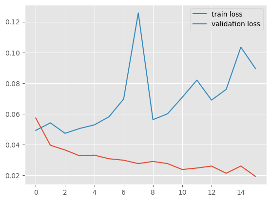

Well, apparently not today, tensorflow.

You can tweak the parameters of the model and perhaps get good metrics, but this game is not worth the candle.

Bonus. Isolation Forest

It would seem that we have done everything possible and after gradient boosting we could stop and say that the model is ready, but for fun we can consider Isolation Forest. It is an unsupervised learning method that is used in clustering and anomaly detection problems.

from sklearn.ensemble import IsolationForest
clf = IsolationForest(max_samples=50, random_state=0)
clf.fit(X_f)
pred=clf.predict(X_f_test)
# на выход модель выдает либо 1 либо -1, для перехода к нашим параметрам, нужно переписать значения:
pred_processed = np.where(pred == -1, 0, pred)

pred_counts = pd.Series(pred_processed).value_counts()

# Строим график
pred_counts.plot(kind='barh', color=sns.palettes.mpl_palette('Dark2'))
plt.gca().spines[['top', 'right']].set_visible(False)
plt.title('Isolation Forest')
plt.xlim(0, pred_counts.max()) 
plt.show()

zeros_count = y_test[y_test == 0].count()
ones_count = y_test[y_test == 1].count()

print("Количество нулей в y_test:", zeros_count)
print("Количество единиц в y_test:", ones_count)

Number of zeros in y_test: koi_pdisposition 894 dtype: int64
Number of units in y_test: koi_pdisposition 1019 dtype: int64

You can run it through metrics, but this does not make much sense, because the number of 0s in real data is approximately 150-200 values ​​higher than in the model, and in principle, the approach of metrics to problems without a teacher is a questionable process. Maybe we didn't get what we were looking for at all.

Conclusion

Gradient boosting remains the thunder of Kaggle and is an excellent model for solving this problem, which did a better job than NN. The reason, it seems to me, is that the neuron needs an order of magnitude more data, and then it will play differently and waiting for the learning process will pay off. I hope that the last 2 articles have interested a certain circle of people, both beginners and more experienced in data science; I would like to receive some feedback on the work done, or some advice on how the model results could be improved.