When a simple Python class is enough – take it and start managing ML experiments
We at Freight One are engaged in cargo transportation, and we solve various transport problems not only using mathematical optimization methods, but also using machine learning models. Our data scientists conduct dozens of experiments, including without the need to resort to logging tools like MLflow. A compact Python class helps them with this. We'll tell you how it works and share the code.

We actively use machine learning to develop solutions that simplify the lives of our employees. For example, we have a “Repair Optimizer”, which helps to draw up a repair plan for wagons and at the same time rank the depot by cost of work. We also use the “Forecaster”, which predicts the volume of cargo transportation between railway stations for subsequent sales planning.
Since we work with dozens of different models, we need to keep track of variables, manage metrics, and compare forecasts. Yes, we use MLflow to version experiments, which offers powerful custom capabilities. We have already talked about this tool on our blog. However, its implementation and support requires working with the infrastructure for logging and monitoring ML experiments, as well as code management.
Simple tasks and small projects don't always require a complex version control solution. If the necessary data is available and the task is clear, then the prototype can be “sketched” in one standard two-week sprint. In other words, in the context of rapid prototyping, when you just need to test a hypothesis, MLflow is definitely overkill.
Just one class
To help data scientists develop prototypes and test hypotheses [причем делать это локально]we have developed a compact tool MLExperimentManager. This is a Python class that provides an interface for loading data, training models, assessing their quality, and logging experimental results. The script makes the process of researching and comparing various ML models more organized and systematized.
from sklearn.datasets import load_iris
from sklearn.model_selection import train_test_split
from sklearn.metrics import accuracy_score, precision_score, recall_score, f1_score, roc_curve, auc, confusion_matrix
from sklearn.ensemble import RandomForestClassifier
from sklearn.linear_model import LogisticRegression
from sklearn.svm import SVC
import seaborn as sns
import pandas as pd
import numpy as np
import matplotlib.pyplot as plt

class MLExperimentManager:
    def __init__(self):
        self.data = None
        self.X_train, self.X_test, self.y_train, self.y_test = (None,) * 4
        self.model = None
        self.experiments_log = None
        self.log_path="experiments_log.csv"

    def load_data(self, dataset):
        self.data = dataset
        X = pd.DataFrame(self.data.data, columns=self.data.feature_names)
        y = pd.Series(self.data.target)
        self.X_train, self.X_test, self.y_train, self.y_test = train_test_split(X, y, test_size=0.2, random_state=42)
        print("Data loaded successfully.")

    def train_model(self, classifier="RandomForest"):
        if classifier == 'RandomForest':
            self.model = RandomForestClassifier(n_estimators=100, random_state=42)
        elif classifier == 'LogisticRegression':
            self.model = LogisticRegression(max_iter=200, random_state=42)
        elif classifier == 'SVC':
            self.model = SVC(probability=True, random_state=42)
        else:
            raise ValueError(f"{classifier} is not supported")
        self.model.fit(self.X_train, self.y_train)
        print(f"Model training completed using {classifier}.")

    def evaluate_model(self, metric="accuracy"):
        predictions = self.model.predict(self.X_test)
        if metric == 'accuracy':
            result = accuracy_score(self.y_test, predictions)
        elif metric == 'precision':
            result = precision_score(self.y_test, predictions, average="macro")
        elif metric == 'recall':
            result = recall_score(self.y_test, predictions, average="macro")
        elif metric == 'f1':
            result = f1_score(self.y_test, predictions, average="macro")
        else:
            raise ValueError(f"{metric} is not a supported metric")
        print(f"Model {metric}: {result}")
        return result

    def log_experiment_to_csv(self, experiment_id, model_params, data_path, result, metric):
        if self.experiments_log is None:
            self.experiments_log = pd.DataFrame({
            'ExperimentID': experiment_id,
            'Comment': 'just_test',
            'Model': self.model.__class__.__name__,
            'ModelParams': str(model_params),
            'DataPath': data_path,
            'Metric': metric,
            'Result': result
        }, index=[0])
        else:
            self.experiments_log = pd.concat([self.experiments_log,
                                             pd.DataFrame({
                                            'ExperimentID': experiment_id,
                                            'Comment': 'just_test',
                                            'Model': self.model.__class__.__name__,
                                            'ModelParams': str(model_params),
                                            'DataPath': data_path,
                                            'Metric': metric,
                                            'Result': result
                                            }, index=[self.experiments_log.index[-1]+1])], ignore_index=True
                                            )

        log_df = pd.DataFrame(self.experiments_log)
        log_df.to_csv(self.log_path, index=False)
        print(f"Experiment {experiment_id} logged successfully to {self.log_path}.")

    # актуально только для бинарной классификации
    def plot_roc_curves(self):
        if hasattr(self.model, "predict_proba"):
            probas_ = self.model.predict_proba(self.X_test)
            fpr, tpr, thresholds = roc_curve(self.y_test, probas_[:, 1])
            roc_auc = auc(fpr, tpr)

            plt.figure()
            plt.plot(fpr, tpr, color="darkorange", lw=2, label="ROC curve (area = %0.2f)" % roc_auc)
            plt.plot([0, 1], [0, 1], color="navy", lw=2, linestyle="--")
            plt.xlim([0.0, 1.0])
            plt.ylim([0.0, 1.05])
            plt.xlabel('False Positive Rate')
            plt.ylabel('True Positive Rate')
            plt.title('Receiver operating characteristic example')
            plt.legend(loc="lower right")
            plt.show()
        else:
            print("The current model does not support probability predictions.")

    def plot_results(self):
        # Предсказываем классы на тестовом наборе
        y_pred = self.model.predict(self.X_test)

        # Считаем матрицу ошибок
        conf_mat = confusion_matrix(self.y_test, y_pred)

        # Визуализируем матрицу ошибок
        sns.heatmap(conf_mat, annot=True, fmt="d", cmap='Blues',
                    xticklabels=self.data.target_names, yticklabels=self.data.target_names)
        plt.xlabel('Predicted labels')
        plt.ylabel('True labels')
        plt.title('Confusion Matrix')
        plt.show()
MLExperimentManager includes several methods:
load_data. The method is responsible for loading data in Parquet/CSV format and provides a convenient interface for pre-processing it, for example, removing gaps. At the same time, it divides the data into training and test sets. The model allows you to conduct tests on data that is beyond the training horizon – that is, on an out-of-time sample (OOT). In other words, her work can be tested on data that she has not seen at all.
train_model. The method is intended for training the model. It supports a variety of algorithms – gradient boosting, random forest, logistic regression, support vector machine. The parameters of the selected model can be optimized – for example, changing the maximum tree depth or modifying the number of trees in the random forest, as well as changing the regularization coefficient in logistic regression.
evaluate_model. Method for assessing model quality. It supports four metrics: accuracy, precision, recall And f1. These are the most common metrics for solving classification problems, but if desired, their number can be expanded.
log_experiment_to_csv. The method is responsible for saving the results of the experiment. They are written to a table that is stored locally. All records contain an experiment identifier, a comment, information about the model used, data, a link to the sample, a metric, the value of this metric on the sample out-of-time and parameters.
plot_roc_curves. A method for visualizing actual and predicted results. It allows you to clearly evaluate the effectiveness of the model, including for colleagues from business units.
You can freely use the MLExperimentManager class in your projects by choosing the necessary parameters in the methods. Just a small note: in its current form, the script is well suited for solving classification problems. If you need to solve regression problems, the code will require modifications. You will have to modify the function train_modeladding algorithms to solve regression problems, and abandon the function plot_roc_curves to visualize the results. You will also need to change the metrics in evaluate_model and rewrite the function plot_results for error calculations for regression problems (for example MAE, MARE, MSE).
Practice
Let's show how to use MLExperimentManager using the famous Iris dataset from the scikit-learn library as an example. It contains information about three species of irises (Iris setosa, Iris virginica and Iris versicolor), and our goal is to train a machine learning model to classify species based on four characteristics: petal and sepal length and width. Let's start by preparing the environment: import the necessary libraries and our MLExperimentManager class, and also load the data.
from sklearn.datasets import load_iris
from MLExperimentManager import MLExperimentManager
iris = load_iris()
Let's initialize and create an instance of the MLExperimentManager class. Let's load Iris data into it, and the script will automatically divide it into training and test samples.
manager = MLExperimentManager()
manager.load_data(iris)
Next, let's move on to training the model: manager.train_model. For example, let's train three different models: random forest (RandomForest), logistic regression (LogisticRegression) and support vector machine (S.V.C.) to compare their effectiveness.
Training a random forest:
manager.train_model(classifier="RandomForest")
manager.evaluate_model(metric="accuracy")
We train logistic regression:
manager.train_model(classifier="LogisticRegression")
manager.evaluate_model(metric="accuracy")
We train the support vector machine:
manager.train_model(classifier="SVC")
manager.evaluate_model(metric="accuracy")
To assess quality we will use manager.evaluate_model with metrics accuracy, precision, recall And f1. Let's immediately write the results to a CSV file:
accuracy = manager.evaluate_model(metric="accuracy")
manager.log_experiment_to_csv(experiment_id=1, model_params=manager.model.get_params(), data_path="iris_dataset", result=accuracy, metric="accuracy")
precision = manager.evaluate_model(metric="precision")
manager.log_experiment_to_csv(experiment_id=2, model_params=manager.model.get_params(), data_path="iris_dataset", result=precision, metric="precision")
f1 = manager.evaluate_model(metric="f1")
manager.log_experiment_to_csv(experiment_id=3, model_params=manager.model.get_params(), data_path="iris_dataset", result=f1, metric="f1")
Let's see what information is recorded in the table:

We use the method plot_roc_curves to visualize the error matrix to better understand how the model classifies different iris species:
manager.plot_results()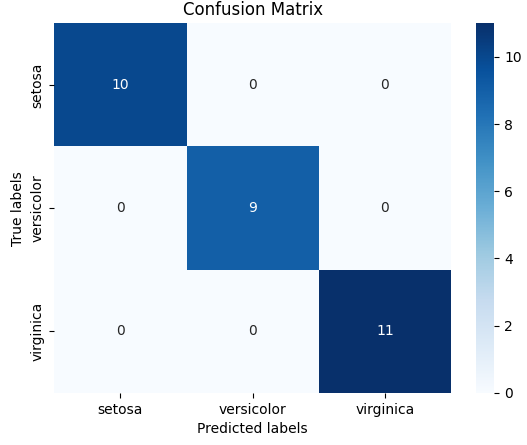
In the graph, the x-axis shows the predicted classes by the model, and the y-axis shows the actual classes. From the error matrix, you can understand that in a specific example the model correctly carried out the classification.
Thus, our MLExperimentManager makes it easy to train multiple models on the Iris dataset and evaluate their quality. And the approach can be easily adapted to work with other data sets and models, making it a valuable tool for machine learning researchers and developers.