Interpolation and discretization, why are they needed for projective image conversion?
The pinhole camera model, which in practice also brings close-up cameras of mobile phones pretty well, tells us that when the camera rotates, images of a flat object are interconnected by projective transformation. The general view of the projective transformation is as follows:
Where projective transformation matrix, and coordinates on the source and converted images.
Geometric Image Conversion
Projective image transformation is one of the possible geometric transformations of images (such transformations in which the points of the original image go to the points of the final image according to a certain law).
To understand how to solve the problem of geometric transformation of a digital image, you need to consider the model of its formation from an optical image on the camera matrix. According to G. Wahlberg [1] Our algorithm should approximate the following process:
- Recover optical image from digital.
- Geometric transformation of the optical image.
- Sampling of the converted image.
An optical image is a function of two variables defined on a continuous set of points. This process is difficult to reproduce directly, because we have to analytically set the type of optical image and process it. To simplify this process, the reverse mapping method is usually used:
- On the plane of the final image, a sampling grid is selected – the points by which we will evaluate the pixel values of the final image (this may be the center of each pixel, or maybe a few points per pixel).
- Using the inverse geometric transformation, this grid is transferred to the space of the original image.
- For each grid sample, its value is estimated. Since it does not necessarily appear at a point with integer coordinates, we need some interpolation of the image value, for example, interpolation by neighboring pixels.
- According to the grid reports, we estimate the pixel values of the final image.
Here, step 3 corresponds to the restoration of the optical image, and steps 1 and 4 correspond to sampling.
Interpolation
Here we will consider only simple types of interpolation – those that can be represented as a convolution of the image with the interpolation core. In the context of image processing, adaptive interpolation algorithms that preserve clear boundaries of objects would be better, but their computational complexity is much higher and therefore we are not interested.
We will consider the following interpolation methods:
- by the nearest pixel
- bilinear
- bicubic
- cubic b-spline
- cubic hermitian spline, 36 points.
Interpolation also has such an important parameter as accuracy. If we assume that the digital image was obtained from the optical method by spot sampling in the center of the pixel and believe that the original image was continuous, then the low-pass filter with a frequency of ½ (see. Kotelnikov theorem)
Therefore, we compare the Fourier spectra of our interpolation cores with a low-pass filter (in the figures are presented for the one-dimensional case).
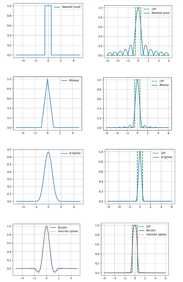
And what, you can just take a kernel with a fairly good spectrum and get relatively accurate results? Actually not, because we made two assumptions above: that there is a pixel value of the image and the continuity of this image. At the same time, neither one nor the other is part of a good model of image formation, because the sensors on the camera’s matrix are not point-like, and on the image a lot of information carries the boundaries of objects – gaps. Therefore, alas, it should be understood that the result of interpolation will always be different from the original optical image.
But you still need to do something, so we will briefly describe the advantages and disadvantages of each of the considered methods from a practical point of view. The easiest way to see this is when you zoom in on the image (in this example, 10 times).
Nearest Pixel Interpolation
The simplest and fastest, however, it leads to strong artifacts.

Bilinear interpolation
Better in quality, but requires more computation and in addition blurs the boundaries of objects.

Bicubic interpolation
Even better in continuous areas, but at the border there is a halo effect (a darker strip along the dark edge of the border and light along the light). To avoid this effect, you need to use a non-negative convolution kernel such as a cubic b-spline.

B-spline interpolation
The b-spline has a very narrow spectrum, which means a strong “blur” image (but also good noise reduction, which can be useful).

Interpolation based on a cubic Hermite spline
Such a spline requires an estimate of the partial derivatives in each pixel of the image. If for approximation we choose a 2-point difference scheme, then we get the core of bicubic interpolation, so here we use a 4-point one.

We also compare these methods in terms of the number of memory accesses (the number of pixels of the original image for interpolation at one point) and the number of multiplication by point.
| Interpolation | Number of pixels | Number of multiplications |
| Near | 1 | 0 |
| Bilinear | 4 | 8 |
| Bicubic | sixteen | 68 |
| B spline | sixteen | 68 |
| Hermite spline | 36 | 76 |
It can be seen that the last 3 methods are significantly more computationally expensive than the first 2.
Sampling
This is the very step to which very little attention has been paid quite undeservedly recently. The easiest way to perform projective image transformation is to evaluate the value of each pixel of the final image by the value that is obtained by inverting its center to the plane of the original image (taking into account the selected interpolation method). We call this approach pixel by pixel sampling. However, in areas where the image is compressed, this can lead to significant artifacts caused by the problem of overlapping spectra at an insufficient sampling frequency.
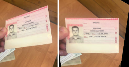
We will clearly demonstrate compression artifacts on the sample of the Russian passport and its individual field – place of birth (Arkhangelsk city), compressed using pixel-by-pixel sampling or the FAST algorithm, which we will consider below.

It can be seen that the text in the left image has become unreadable. That’s right, because we take only one point from a whole region of the source image!
Since we were not able to estimate by one pixel, then why not choose more samples per pixel, and average the obtained values? This approach is called supersampling. It really increases the quality, but at the same time, the computational complexity increases in proportion to the number of samples per pixel.
More computationally efficient methods were invented at the end of the last century, when computer graphics solved the problem of rendering textures superimposed on flat objects. One such method is conversion using mip-map structure. Mip-map is a pyramid of images consisting of the original image itself, as well as its copies reduced by 2, 4, 8 and so on. For each pixel, we evaluate the degree of compression characteristic of it, and in accordance with this degree we select the desired level from the pyramid, as the source image. There are different ways to evaluate the appropriate level of mip-map (see details [2]) Here we will use the method based on the estimation of partial derivatives with respect to the well-known projective transformation matrix. However, in order to avoid artifacts in areas of the final image where one level of the mip-map structure changes to another, linear interpolation is usually used between two adjacent levels of the pyramid (this does not greatly increase the computational complexity, because the coordinates of the points at neighboring levels are uniquely connected).
However, the mip-map does not take into account the fact that image compression can be anisotropic (elongated along some direction). This problem can be partially solved. rip-map. A structure in which images compressed in times horizontally and times vertically. In this case, after determining the horizontal and vertical compression coefficients at a given point in the final image, interpolation is performed between the results of 4 copies of the original image compressed at the desired number of times. But this method is not ideal, because it does not take into account that the direction of anisotropy differs from directions parallel to the boundaries of the original image.
The algorithm partially solves this problem. Fast (Footprint Area Sampled Texturing) [3]. It combines the ideas of mip-map and supersampling. We estimate the degree of compression based on the axis of least anisotropy and select the number of samples in proportion to the ratio of the lengths of the smallest axis to the largest.
Before comparing these approaches in terms of computational complexity, we make a reservation that in order to accelerate the calculation of the inverse projective transformation, it is rational to make the following change:
Where , Is the matrix of the inverse projective transformation. As and functions of one argument, we can pre-calculate them for a time proportional to the linear size of the image. Then, to calculate the coordinates of the inverse image of one point of the final image , only 1 division and 2 multiplications are required. A similar trick can be performed with partial derivatives, which are used to determine the level in the mip-map or rip-map structure.
Now we are ready to compare the results in terms of computational complexity.
| Method | The number of samples per pixel | The number of multiplications per count | Additional memory for structures (in fractions of the original image) |
| Pixel Sampling | 1 | 2 | 0 |
| Supersampling | n | 2 | 0 |
| Mip-map | 2 | 7 | 1/3 |
| Rip map | 4 | 7 | 3 |
| Fast | <= n | 7 | 1/3 |
And compare visually (from left to right pixel-by-pixel sampling, supersampling by 49 samples, mip-map, rip-map, FAST).

Experiment
Now, let’s compare our results experimentally. We compose a projective transformation algorithm combining each of 5 interpolation methods and 5 discretization methods (25 options in total). Take 20 images of documents cropped to 512×512 pixels, generate 10 sets of 3 projective transformation matrices, such that each set is generally equivalent to the identity transformation and we will compare the PSNR between the original image and the converted one. Recall that PSNR is where this is the maximum in the original image a – the standard deviation of the final from the original. The more PSNR the better. We will also measure the operating time of projective conversion on ODROID-XU4 with an ARM Cortex-A15 processor (2000 MHz and 2GB RAM).
Monstrous table with the results:
| Sampling | Interpolation | Time (sec.) | PSNR (dB) |
| Pixel by pixel | Near | 0.074 | 23.1 |
| Bilinear | 0.161 | 25.4 | |
| Bicubic | 0.496 | 26.0 | |
| B spline | 0.517 | 24.8 | |
| Hermite spline | 0.978 | 26.2 | |
| Supersampling (x49) | Near | 4.01 | 25.6 |
| Bilinear | 7.76 | 25.3 | |
| Bicubic | 23.7 | 26.1 | |
| B spline | 24.7 | 24.6 | |
| Hermite spline | 46.9 | 26.2 | |
| Mip-map | Near | 0.194 | 24.0 |
| Bilinear | 0.302 | 24.6 | |
| Bicubic | 0.770 | 25.3 | |
| B spline | 0.800 | 23.9 | |
| Hermite spline | 1.56 | 25.5 | |
| Rip map | Near | 0.328 | 24.2 |
| Bilinear | 0.510 | 25.0 | |
| Bicubic | 1.231 | 25.8 | |
| B spline | 1.270 | 24.2 | |
| Hermite spline | 2.41 | 25.8 | |
| Fast | Near | 0.342 | 24.0 |
| Bilinear | 0.539 | 25.2 | |
| Bicubic | 1.31 | 26.0 | |
| B spline | 1.36 | 24.4 | |
| Hermite spline | 2.42 | 26.2 |
What conclusions can be drawn?
- The use of interpolation by the nearest pixel or pixel-by-pixel sampling results in poor quality (it was obvious from the examples above).
- Interpolation by Hermite polynomials over 36 points or supersampling are computationally expensive methods.
- Using bicubic or b-spline interpolation with any discretization method other than pixel-by-pixel also takes a lot of time.
- Rip-map is comparable to FAST in terms of operating time, while its quality is slightly worse, and it draws 9 times more additional memory (the choice is obvious, right?).
- Discretization using mip-map and interpolation with b-spline demonstrated low PSNR because they cause relatively strong blurring of the image, which is not always such a serious problem.
If you want good quality with not too low speed, you should consider bilinear interpolation in combination with discretization using mip-map or FAST. However, if it is known for certain that projective distortion is very weak, to increase the speed, you can use pixel-by-pixel discretization paired with bilinear interpolation or even interpolation by the nearest pixel. And if you need high quality and not very limited run time, you can use bicubic or adaptive interpolation paired with moderate supersampling (for example, also adaptive, depending on the local compression ratio).
P.S. The publication is based on the report: A. Trusov and E. Limonova, “The analysis of projective transformation algorithms for image recognition on mobile devices,” ICMV 2019, 11433 ed., Wolfgang Osten, Dmitry Nikolaev, Jianhong Zhou, Ed., SPIE, Jan. 2020, vol. 11433, ISSN 0277-786X, ISBN 978-15-10636-43-9, vol. 11433, 11433 0Y, pp. 1-8, 2020, DOI: 10.1117 / 12.2559732.
- G. Wolberg, Digital image warping, vol. 10662, IEEE computer society press Los Alamitos, CA (1990).
- J. P. Ewins, M. D. Waller, M. White, and P. F. Lister, “Mip-map level selection for texture mapping,” IEEE Transactions on Visualization and Computer Graphics4 (4), 317–329 (1998).
- B. Chen, F. Dachille, and A. E. Kaufman, “Footprint area sampled texturing,” IEEE Transactions on Visualization and Computer Graphics10 (2), 230–240 (2004).
Similar Posts