Improving the RandomForestClassifier model
Article taken from source Daily Dose of Data Science.
I’ll make a reservation right away: I’m new to Data Science and to the design of articles. I’m only writing here for my notes and maybe it will be useful to someone. Please don’t judge too much!)
Random Forest is a fairly powerful and robust model that is a combination of many different decision trees.

But the biggest problem is that whenever we use random forest, we always create many more underlying decision trees than required.
Of course, this can be tuned using hyperparameters, but this requires training many different random forest models, which takes a lot of time.
And in this article I share one of the most incredible techniques that I recently discovered for myself:
Improving the accuracy of the random forest model.
We reduce the size of the RandomForestClassifier model.
We radically reduce the time for prediction.
And all this without having to retrain the model.
Logics
We know that a random forest model is a collection of many different decision trees:
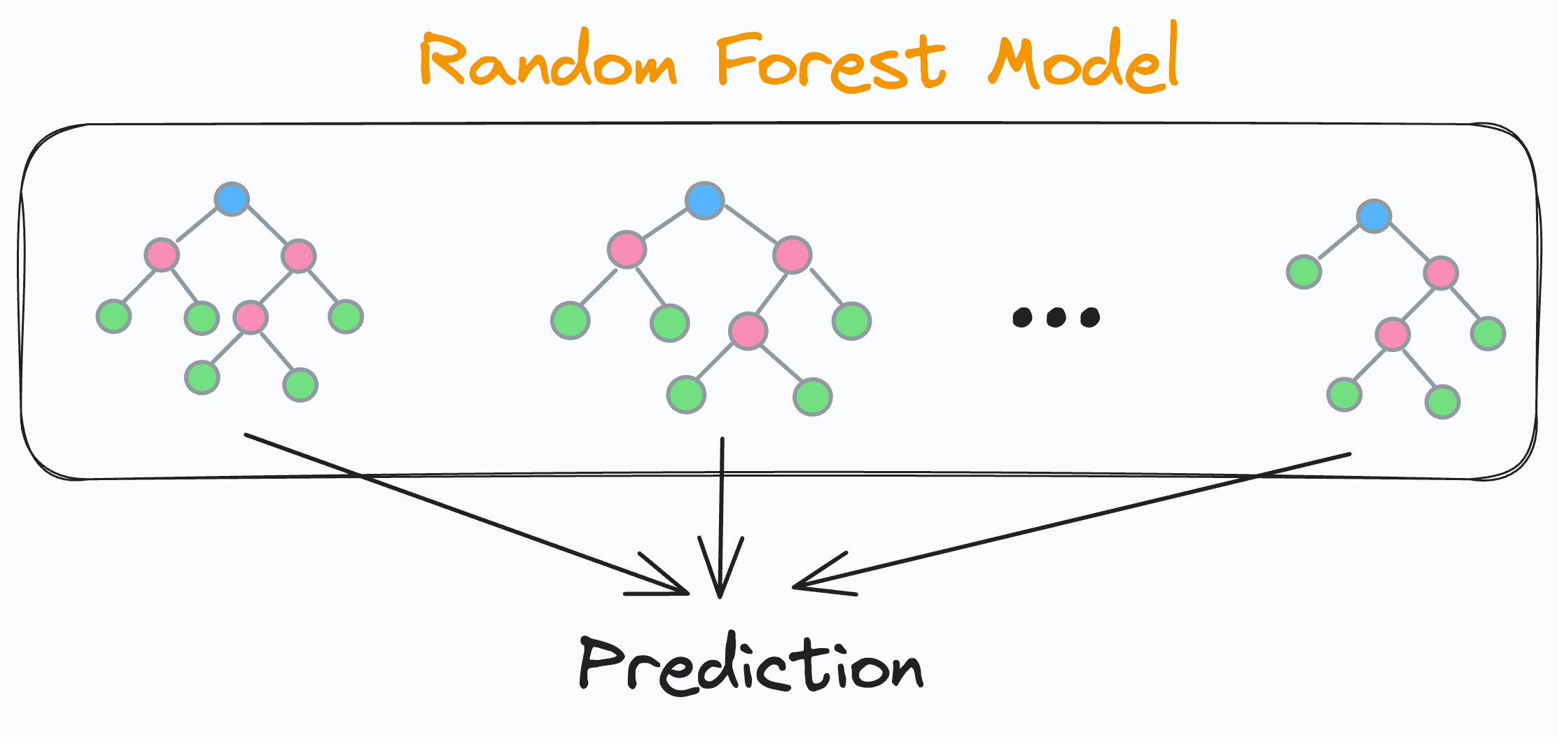
The final prediction is generated by combining the predictions from each separate and independent decision tree. Since each decision tree in a random forest is independent, this means that each decision tree will have its own accuracy on the test data, right?
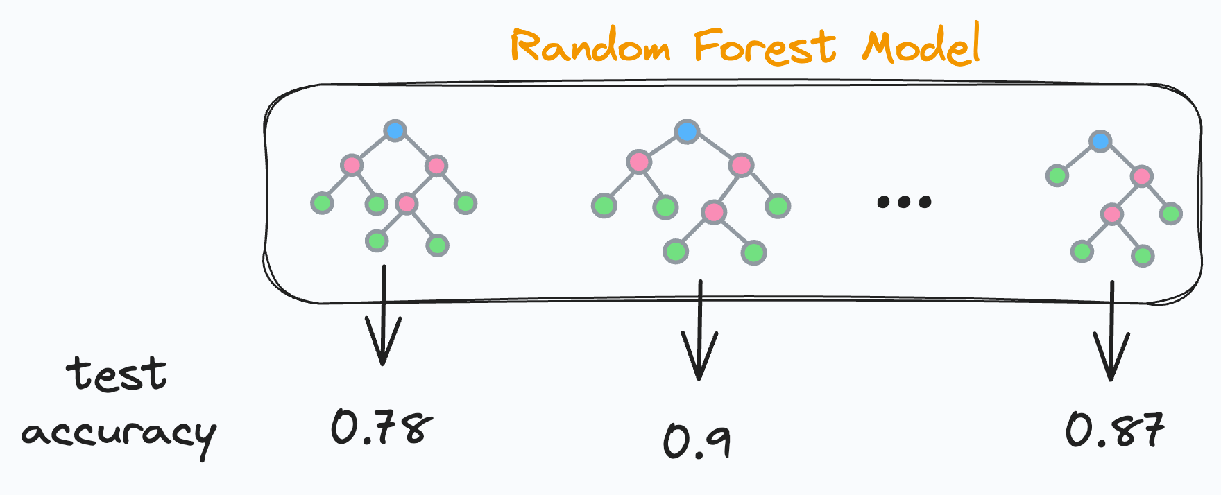
But this also means that some decision trees show worse results and some show better results. Right?
So what if we do the following:
We will find the accuracy on test data for each decision tree.
We will sort the precisions in descending order.
We will keep only the “k” best decision trees and remove the rest.
After this, only the decision trees with the best results evaluated on the test data set will remain in our random forest. Cool, isn’t it?
Now, how to determine the “k” best trees?
It’s simple.
We can plot the cumulative accuracy.
This will be a line graph showing the accuracy of the random forest:
Considering only the first two decision trees.
Considering only the first three decision trees.
Considering only the first four decision trees.
And so on.
Accuracy is expected to initially increase with the number of decision trees and then decrease.
By looking at this graph, we can find the most optimal “k” decision trees.
Implementation
Let’s look at its implementation.
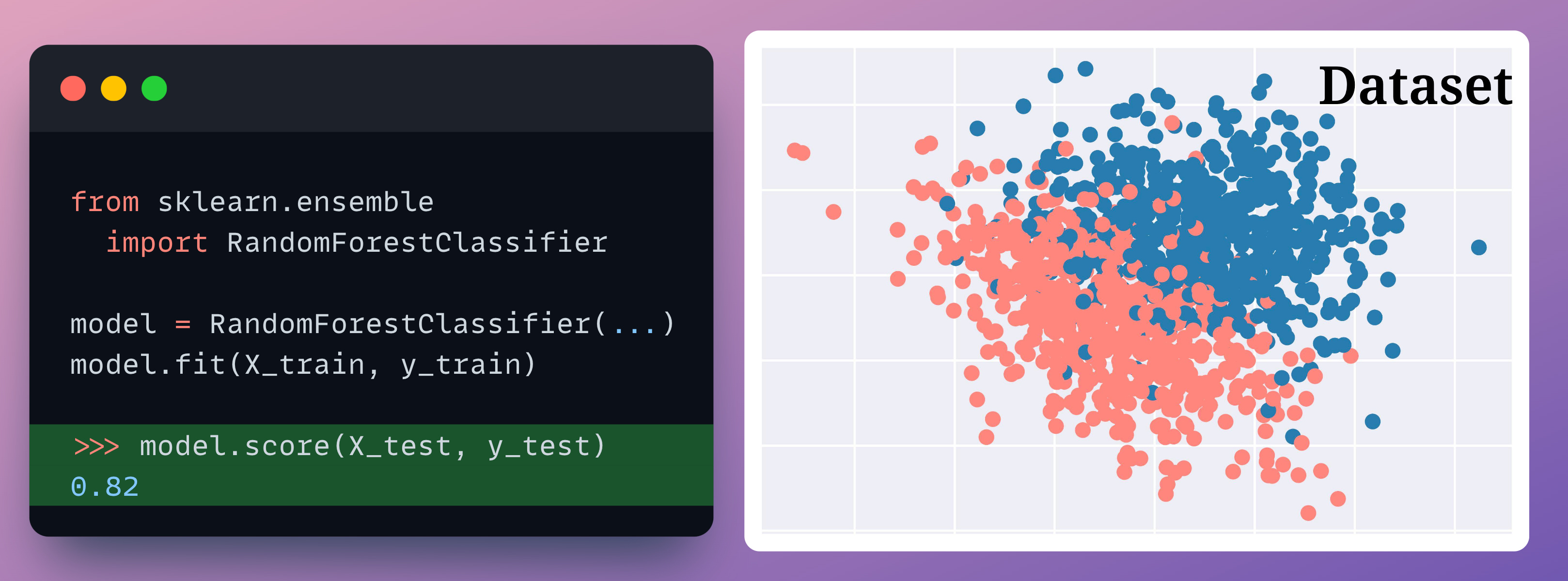
First we train our random forest as usual:
Next, we must calculate the accuracy of each decision tree model.
In sklearn, individual trees can be accessed using the model.estimators_ attribute.
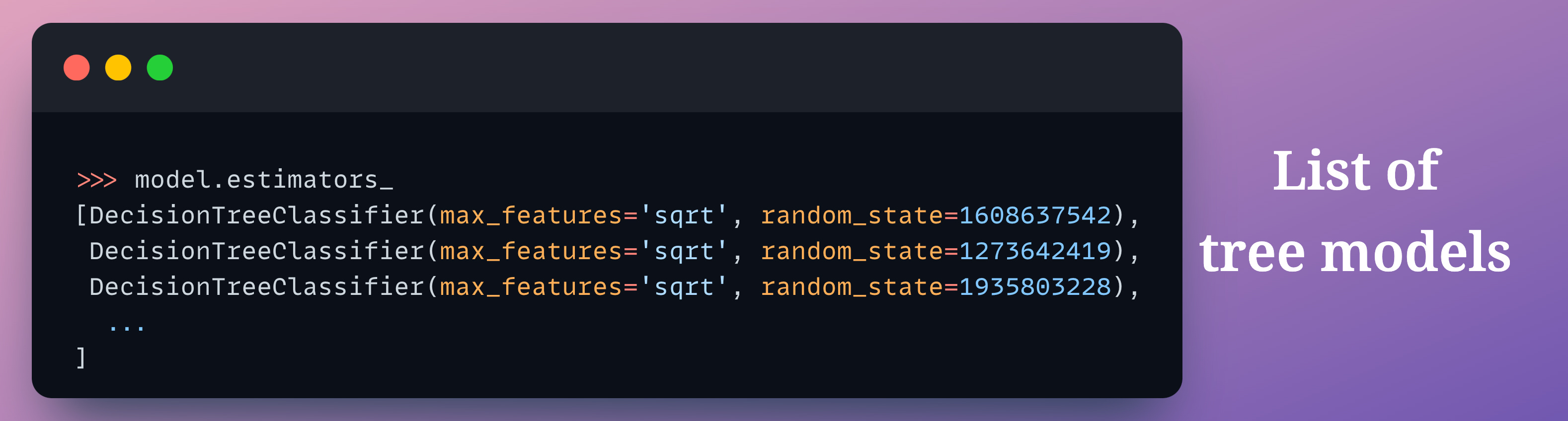
Thus, we iterate over all the trees and calculate their testing accuracy:

model_accs is a NumPy array that stores the tree ID and its testing accuracy:
>>> model_accs
array([[ 0.   ,  0.815], # [tree id, test accuracy]
       [ 1.   ,  0.77 ],
       [ 2.   ,  0.795],
          ...
Now we must rearrange the decision tree models in the model.estimators_ list in descending order of testing accuracy:
# sort on second column in reverse order to obtain sorting order >>> sorted_indices = np.argsort(model_accs[:, 1])[::-1]

# obtain list of model ids according to sorted model accuracies >>> model_ids = model_accs[sorted_indices][:,0].astype(int) array([65, 97, 18, 24, 38, 11,...
Этот список сообщает нам, что 65-я индексированная модель является самой производительной, за ней следует 97-я индексированная и так далее ….
Теперь давайте переставим модели деревьев в списке model.estimators_ в порядке model_ids:
# create numpy array, rearrange the models and convert back to list
model.estimators_ = np.array(model.estimators_)[model_ids].tolist()
Made!
Finally, we create the plot discussed earlier.
This will be a line graph showing the accuracy of the random forest:
Considering only the first two decision trees.
Considering only the first three decision trees.
Considering only the first four decision trees.
and so on.
Below is the code to calculate the cumulative precision:

In the above code:
We create a copy of the base model called small_model.
At each iteration, we set small_model trees to the first “k” trees of the base model.
Finally, we evaluate small_model using only “k” trees.
By plotting the cumulative accuracy result, we get the following graph:

The graph shows that the maximum accuracy of the test is achieved when considering only 10 trees, which means a tenfold reduction in the number of trees.
Comparing their accuracy and execution time, we get:
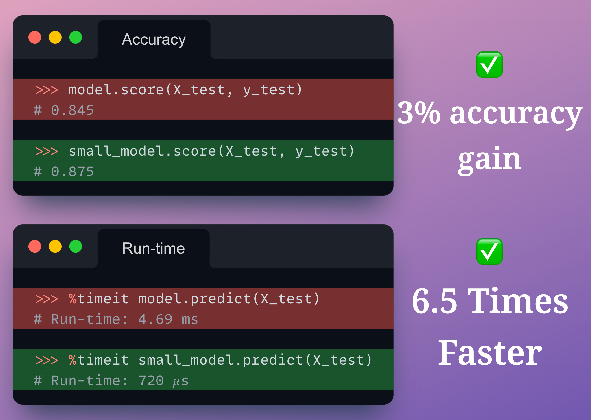
We get a 3% increase in accuracy.
execution time for prediction is 6.5 times faster.
Note that:
We did not retrain and select hyperparameters
By selecting the best trees, we reduced the training time
And that’s cool!
You can download this notebook here: Jupyter Notebook.
That’s all! Thanks for reading! Article taken from source Daily Dose of Data Science.
What other solutions are there? Write comments!