two statistics with similar names but different meanings
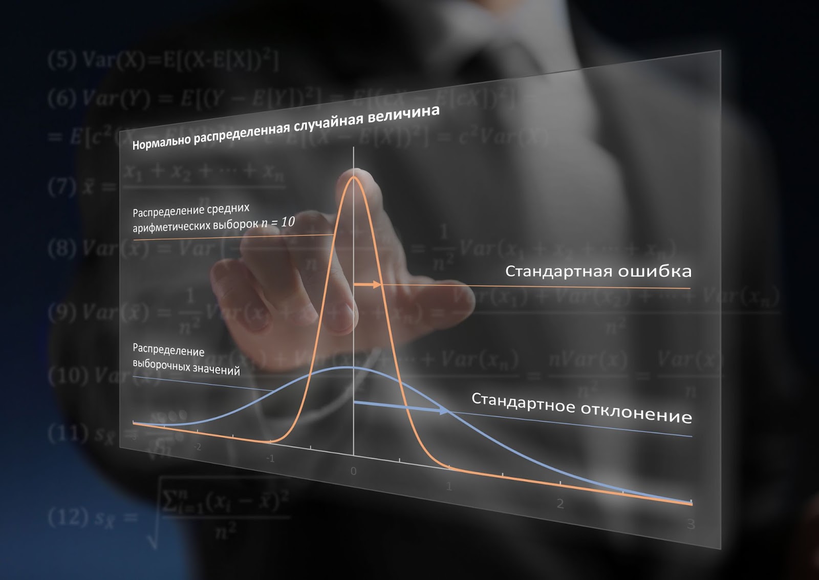
I teach a course on statistical thinking to masters, and one topic causes obvious difficulties for them – how the standard deviation differs from the standard error and in what cases to apply this or that statistics. I think it will be interesting to talk about this on the LANIT blog.
Random variables
Let – random normally distributed variable. Its mathematical expectation in probability theory is denoted
or
and in statistics –
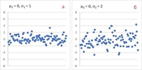
. Let's create two samples of 100 values each. To generate samples in Excel, we use the formula =NORM.REV(RAND();
;
). Let's set the same expectations
and different standard deviations:
And
.
Arithmetic mean of the sample
Despite the fact that we have set the expectation for the generating process , the sample average will differ from this value. The sample average is called arithmetic mean
(or just average), and calculated using the formula:
Where – individual values of a random variable,
– number of random variable values in the sample.
For the samples in Fig. 1 it turned out that ,
.
Dispersion and standard deviation of the population
To measure the dispersion (variability) of a random variable relative to its expectation, the dispersion is most often used, denoted ,
or
… and standard deviation
Sample standard deviation
Standard Deviation (SD) calculated by the formula:
In general, terms are used slightly differently by different authors. I like the following approach. The population is described parametersdenoted by Greek letters: mathematical expectation and standard deviation
. Samples describe statisticiansdenoted by Latin letters: arithmetic mean
and standard deviation
.
In real life, no mathematical expectation nor standard deviation σ general population are unknown. But by extracting a sample, we learn something about expectation and standard deviation. They say it's average
is assessment mathematical expectations
and the standard deviation
– assessment standard deviation σ.
When generating a random variable, we set And
. For the samples in Fig. 1 received
,
.
The less , the more closely the values are located around the average. So,
standard deviation – a measure of the spread of data in a sample
Standard Deviation of Sample Means
Let us now focus on the process of generating random numbers with And
. Let's extract not just one sample, but several. Although the arguments
And
random number generator are constant, the random process will lead to different values
for individual samples:

If we take not 15, but 1000 samples, we can build a fairly smooth distribution of average values :
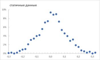
Set of averages can be considered as a random variable
. For its distribution (Fig. 3), you can also calculate the standard deviation using formula (4):
. Subscript
indicates that the standard deviation refers to the average values
. Note that the standard deviation of one sample (Fig. 1a) was equal to
. The standard deviation of each sample is given by the generating process, in which the standard deviation of the population
. For average values of samples of size
standard deviation
approximately 10 times less than for individual values in the sample
.
Let's calculate the standard deviation for 100 samples of other sizes . It turns out that the standard deviation of the means depends on the sample size:
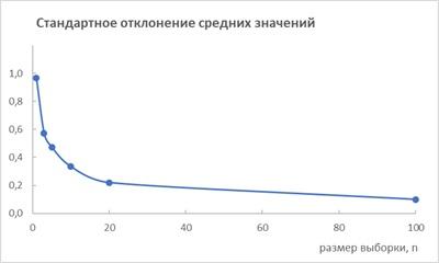
Let us derive the formula for this dependence.
Standard error formula
To begin with, we will show that the constant factor can be taken out of the dispersion sign by squaring it.
By definition, variance random variable
equal to
Where – mathematical expectation of a random variable
– mathematical expectation of the squared difference between the random variable itself and its expectation.
Let us now consider the random variable Where
– constant. Let's find the variance
On the other hand, the arithmetic mean for the sample:
Sample variance:
Here we have taken advantage of the property (6) we just derived, using .
Now let’s take into account that the variance of the sum of independent random variables is equal to the sum of their variances:
Let us take into account that all random variables equally distributed:
By taking the root and moving from the population parameter to the sample statistics, we can write the standard deviation of the random variable :
We obtained the dependence of the standard deviation of the average values of the samples from standard deviation of single values
and sample size
. If we substitute (4) into (11), we get:
Sizecalled standard error or standard error of the mean.
allows you to estimate from one sample in what range from the sample average
the mathematical expectation of the general population is found
. For example, in the range
the expectation of the general population will hit with a probability of 95%.
If the standard deviation is an indicator of the variability of elements in a sample, then the standard error is a similar indicator (calculated using the same formula) of the variability of sample means.
So,
standard error – a measure of the mathematical expectation of the population μ based on the sample mean .
Note that as sample size increases the standard error will decrease. In the limit at
,
And
.
Biased and unbiased estimates
The estimate of the population parameter in the general case can be represented by the equation:
(13) Estimate = Estimated Population Parameter + Bias + Noise
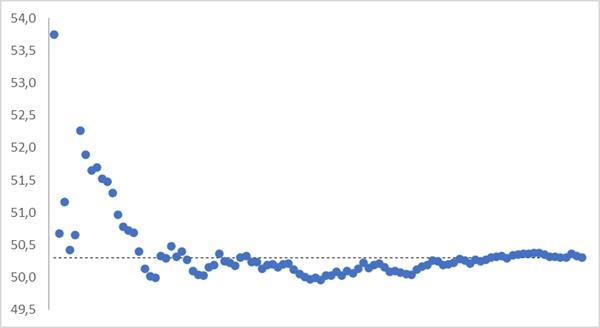
It turns out that the arithmetic mean is an unbiased estimate of the expectation:
To illustrate this point, I randomly assigned 10,000 numbers ranging from 0 to 100. And then created 100 samples of 100 consecutive values: from 1 to 100, from 101 to 200, etc. The average value for all 10,000 random numbers is plotted on the graph in the form of a dotted line, as well as the moving average for a sequence of samples in the form of dots. For example, the first point is the arithmetic mean for the first sample: 1…100, the second point is the statistical average of two samples: 1…100 and 101…200, etc.
It seems paradoxical, but the standard deviation turned out to be a biased estimate of the standard deviation:
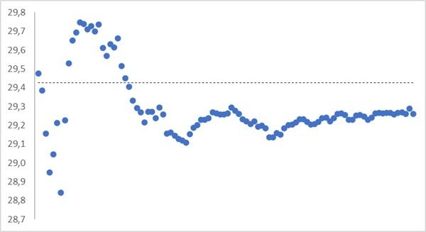
A sample estimate of the standard deviation, which we called the standard deviation, and introduced by formula (4) gives a systematic error!
Bessel amendment
To understand the source of systematic error, we once again present the formulas for root mean square and standard deviation.
… and let's return to the example in Fig. 1a.
We know (we set it ourselves in Excel) that the expectation of the general population . But the arithmetic mean of the sample
. And this is our best estimate of the expectation. Correct (unbiased) estimate of the population standard deviation σ should be based on deviations from
according to formula (3). But if we don't know the true meaning
then we calculate the standard deviation
from
according to formula (4).
notice, that in formula (3) can be represented as
Where
– a constant (bias) indicating how much the sample mean differs from the expectation of the general population. Then
can be replaced by
. Let's denote the difference
one character
. In formula (4) we are looking for the sum
and in formula (3) – the sum
. But
By definition, the sum of the second terms over the sample is equal to zero – deviations from the average in different directions compensate each other. That's why it's average. Sum
is the sum of the squares of the distance from the sample values to the sample mean.
– the sum of squared distances between the arithmetic mean of the sample and the expectation of the general population.
Because the positive (except when
) the sum of the squares of the distance from the sample values to the population expectation will always be greater than the sum of the squares of the distance to the sample mean.
That's why gives a systematic error (downward) compared to
.
In a biased estimate , By using the sample mean instead of the expected value, we underestimate each
on
.
To find the discrepancy between the biased estimate and population parameter σwe need to find the expectation
. In chapter Standard error formula we showed that this expectation is equal to the variance of the sample mean σ/n. Thus, the biased estimate underestimates
on
:
biased estimate
unbiased estimate
unbiased estimate
The Bessel correction is the coefficient by which the standard deviation should be multiplied to make the biased estimate unbiased:
Let's check the behavior on model:
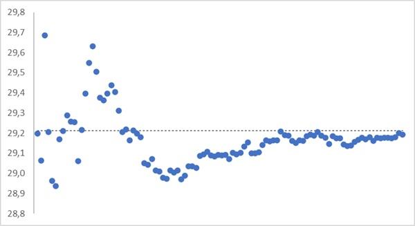
The Bessel correction should also be introduced into formula (12) to calculate the standard error of the mean. We get:
Assumptions
When deriving the standard deviation and standard error formulas, we used the following assumptions, either explicitly or implicitly:
the data in the sample is subject to normal distribution;
sample is representative for the general population;
observations in the sample independent from each other; for time series, the assumption of independence is usually violated;
measurements are carried out on interval or relative scale; the use of categorical data may be incorrect;
assessments sensitive to emissions.
Let's see what happens when one or more assumptions are violated.
Distributions with fat tails
The normal distribution has a thin tail. This means that the behavior of a normally distributed random variable is determined by the central part of the distribution. Tail values are very rare. Central limit theorem gives fast convergence, and we observe characteristic behavior as in Fig. 5.
In response to my query, ChatGPT pointed out three areas where the data is well described by a normal distribution: human height, measurement errors (of length or mass among a homogeneous group of objects), intellectual ability (IQ tests are designed to fit a normal distribution, and average intelligence tends to fall in the middle distributions).
The normal distribution is so widespread that we use it even when we shouldn’t – when working with financial instruments, economic and social phenomena. A typical example is the average income of bar patrons, which will skyrocket to a billion if Bill Gates happens to walk in there.
Let's see how a random variable defined by the standard Cauchy distribution converges to the mean:
To model in Excel, I took advantage of the fact that the Student t-distribution with the number of degrees of freedom is equivalent to the standard Cauchy distribution. And for t-Student in Excel there are formulas for direct and inverse distributions.
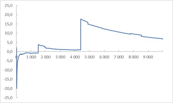
If we look at the assumptions stated above, we see that Cauchy distributed data violates almost everything. (1) No sample is representative. The tail values are still relatively rare (though not as rare as in a normal distribution), but they determine the sample average. (2) Presence or absence emission in a sample, the arithmetic mean has a stronger effect than central tendency.
Following the arithmetic mean, both the standard deviation and the standard error obtained from a sample tell little about the population.
I used the extremely fat-tailed Cauchy distribution as an example, but many other distributions, such as power-law ones, behave only slightly more predictably. This topic is covered in detail in Nassim Taleb's new book (see link below).
Areas of use
Here are some uses of standard deviation:
Estimation of data scatter (variability) relative to the average value. The larger the standard deviation, the greater the spread.
Quality control as an indicator of variability in the production or management process. A smaller standard deviation indicates a more stable process. Standard deviation can be used to plot boundaries Shewhart control charts.
Areas of use of Standard Error of the Mean (SEM):
Confidence intervals for the mean. For example, if you conducted a survey with a small sample and calculated the mean and SEM, you can construct a confidence interval indicating where the true mean lies in the population.
When comparing average values from different samples SEM is used to determine the statistical significance of differences between samples. If the difference in means is greater than a few SEMs, it may indicate a statistically significant difference.
SEM indicates how accurate The sample mean estimates the true mean of the population. A large SEM indicates greater uncertainty in the estimate.
With caution and reservations, standard deviation and standard error should be used to assess risk in the financial sector. The SD and SEM formulas are based on several statistical assumptions. It is important to understand these assumptions when using and interpreting the results.
Literature
Vladimir Gmurman. Theory of Probability and Mathematical Statistics
Bessel amendmentBessel's correction
Nassim Nicholas Taleb. Statistical implications of fat tails.


