Spark. Query plan with examples
Hi all!
In this article, we’ll take a couple of tables as a basis and go through query plans incrementally: from regular select to joins, windows and repartitioning. Let's see how the types of plans differ from each other, what changes in them from query to query, and let's look at each line using the example of a partitioned and non-partitioned table.
Initial data
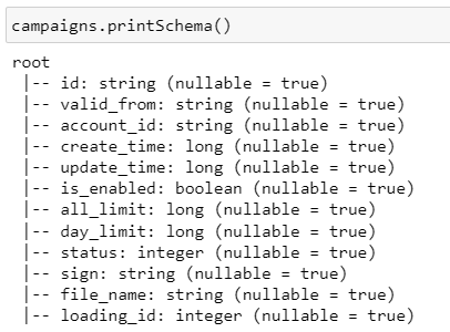
We will work with 3 tables:
1) campaigns – partitioned by loading_id field
2) campaigns_not_partitioned – exactly the same table, but not partitioned
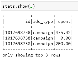
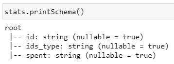
3) stats – table with which we will test joins

Briefly about the types of plans
There are 4 plans in total:
Parsed Logical Plan – plan after parsing a cell with code, catches syntax errors
Analyzed Logical Plan – plan after semantic analysis, specific tables and columns with data types are pulled up
Optimized Logical Plan – optimization to the previous plan, for example, simplifies unnecessary operations to improve performance
Physical Plan – how the request will be physically executed on the cluster, specific files, paths, formats, partitions, etc.
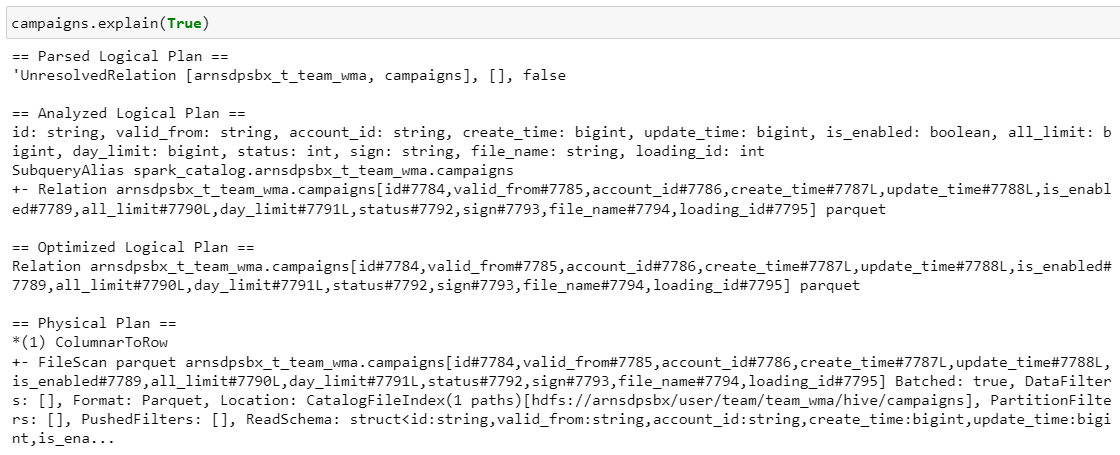
Further we will look only at the physical plane, because it reflects the actual data processing algorithm. To make reading comfortable, there is a table of contents with quick links to the queries themselves.
Let's go!
Table of contents
1. The most common selection

Well, let's go study the plan:
1) FileScan parquet
Our table is read from the schema, all fields are listed, the data format is parquet, which is stored on hdfs along the specified path, there are no partitions (in this case we take everything), there are no filters, the data schema is indicated.
2) ColumnarToRow
The source data is stored in parquet files column by column, but in spark the dataframe essentially contains many rows, so we need to convert columns to rows.
Let me remind you that the first table was partitioned by the loading_id field. Now let's look at a non-partitioned table:

What has changed?
Location instead CatalogFileIndex became InMemoryFileIndex.
CatalogFileIndex used when we read the entire partitioned table.
InMemoryFileIndex used when we are reading a non-partitioned table or individual partitions.
2. The most common filter

As we can see, the field has been filled PartitionFilters – we selected specific partitions. In general, the Catalyst optimizer always adds one more filter in its filters – isnotnullbecause in order to filter by specific values, the field must definitely not be empty.
In a non-partitioned table:

PartitionFilters moved to a level DataFilters And PushedFilters.
DataFilters – these are filters on non-partitioned columns.
PushedFilters – filters that we can forward to the data source level and apply directly when reading a file.
However, these two parameters may not coincide. Here I added a purely technical filter:

IN DataFilters there is a filter with concat(), and in PushedFilters no longer exists, because we cannot apply this complex construction at the source.
Also, one more step is added to the query plan – Filter. It is needed to finally filter the data according to the specified conditions. Because at the stage PushedFilters we don't take necessary lines, and we take files containing the required lines. Accordingly, something extra can easily get into them.
3. Select one column

In the case of a partitioned table, we will always drag the partitioning field along with us, and then execute Project – That's what it is select.
4. Select one column + filter
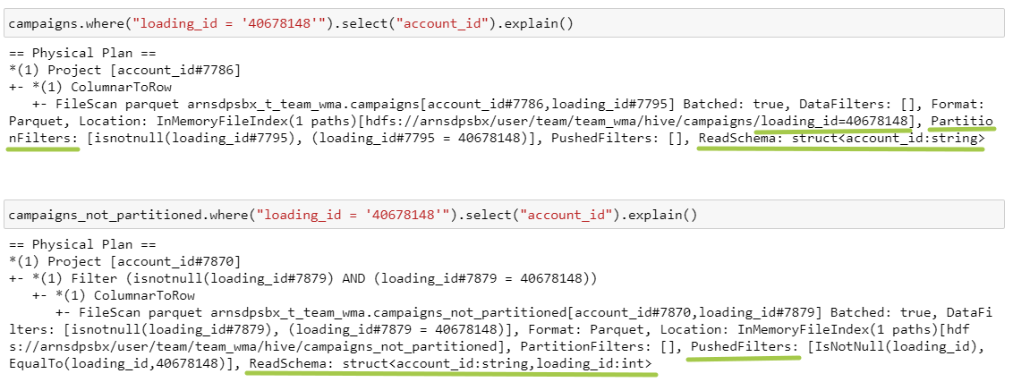
Besides the difference between PartitionFilters And PushedFilterswhich we have already discussed in paragraph 2, a difference in the parameter has also been added ReadSchema. If the table is partitioned, then the partitioning field is not stored as a column in the data, it is moved to the file system level: therefore, in the first path there is a folder /loading_id=40678148. In the second case, loading_id is stored directly in the file, so we need to get it first.
5. Caching

2 operations have been added here: InMemoryRelation, InMemoryTableScanwhich will always accompany any transformation with a cached table.
So, we looked at the most under-the-hood things, there will be no more differences between the tables. Next, I will insert only the actions themselves, so as not to fill the screen with the same type of information, and leave the set of columns, diagrams, etc. outside the brackets.
6. Renaming, adding a new column
Both pairs of queries lead to the same result, operations are performed at the stage Project:


7. Select with functions, case when


The use of functions, case when, as well as changing the naming of fields, occurs at the stage Project.
8. Grouping


Since for grouping we need only one account_id field, and spark for each subsequent stage wants to transfer as little data as possible, then in FileScan we take only the required fields. Operation Project appeared due to the fact that we are still dragging behind us the field of partitioning.
Now let's look at the new operations:
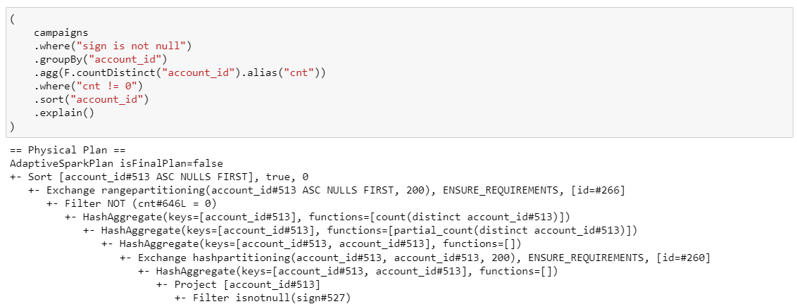
HashAggregate – aggregation, keys – grouping fields, functions – aggregating function. Partial_count is used here because Spark tries to do aggregation in 2 approaches:
1 – aggregation within each partition.
Exchange hashpartitioning – this is a shuffle, 200 is the number of parts after the shuffle. All identical keys are collected within one partition based on hash code calculation, and key-partial_count pairs are exchanged.
2 – second iteration of aggregation, all partial_counts are summed up.
9. Distinct

The only difference distinct from groupBy – this is the absence of an aggregation function.
10. Sort

Exchange range partitioning – at this stage, the data is distributed based on the range. For example, if account_id is from 1 to 100 and we want to divide it into 3 partitions, then account_id from 1 to 33 will fall into the first partition, from 34 to 66 – into the second, and then by analogy.
11. Aggregation functions

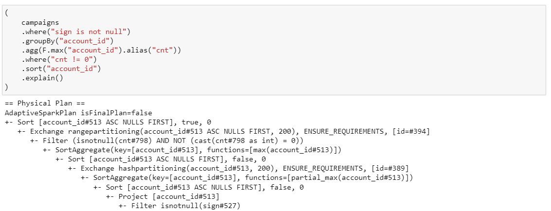
Here we see a new stage – SortAggregate. It is used when HashAggregate is not possible due to memory limitations or when it does not support aggregation functions or keys (for example, immutable data types, and in our example both fields are of type string). This method involves pre-sorting and is therefore slower. SortAggregate as well as HashAggregateis performed in 2 approaches: before the shuffle locally on each mapper and after the shuffle.
And since we are counting the minimum value, the corresponding functions partial_min and min are used.
Let's try to remove the grouping:

One of our stages has changed: Exchange SinglePartition. This means that all data is moved to one partition and will be processed on one core. It is used when calculating, for example, min, max, avg or with a window without a partitioning key (bad!).
12. DropDuplicates

Function dropDuplicates if there are duplicates, by default it leaves the first element, so partial_first is considered first within each partition, and after the shuffle first for each key. Everything as usual.
13.Window functions

It seems that, taking into account the previous points, everything is already quite simple: we do not need to pre-aggregate or sort, so we start immediately with the shuffle stage. Then the .orderBy() part is executed, the window function is calculated, and the specified selection of fields is taken. All other windows are similar, only the stage changes Window.
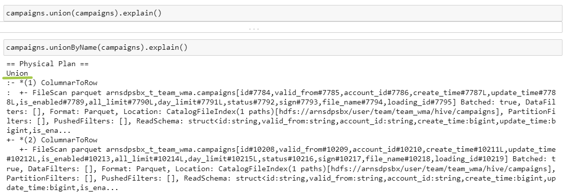
14.Union
Both queries lead to the same result, two tables are read, which are then joined in the step Union:
15.Join
SortMergeJoin

SMJ works when there is an equality condition and when the keys are sortable.
What's happening?
Filter isnotnull: Since we have an inner join, the keys cannot contain null, so Spark filters as early as possible in order to process less data.
A small table on the types of joins:
Join type | Left filter available | Availability of right filter | A comment |
inner | + | + | both keys are not null |
left | – | + | the left table may contain null |
right | + | – | the right table may contain null |
full | – | – | both tables can contain null |
Exchange hashpartitioning – both dataframes are repatriated into 200 partitions using the join keys.
Sort – sorting within the partition by join keys.
SortMergeJoin – the loop goes through each pair of partitions, and by comparing the left and right keys, rows with the same keys are connected.
ShuffledHashJoin

SHJ only works if there is a hint, because the default is SMJ. In this case we are missing a stage Sort and the appearance of the join changes.
Exchange hashpartitioning – dataframes with the same join key are moved to one executor.
ShuffledHashJoin – a hash table is created on the executor for a smaller dataframe, where the key is a tuple of join fields (in our example, id). It then iterates through the larger dataframe within each partition and checks for the presence of keys in the hash table.
BroadcastHashJoin

BHJ works when there is a condition on equality and when one of the dataframes is small and fits completely into the executor’s memory.
BroadcastExchange – this is copying the right dataframe to each executor.
Hash join occurs in a similar way, the main difference is in the use of data exchange strategy: shuffle for SHJ and broadcast for BHJ.
BroadcastNestedLoopJoin

BNLJ works when there is a condition on inequality and when one of the dataframes is small and fits completely into the executor’s memory.
BroadcastNestedLoopJoin – in a nested loop we go through the elements of each partition of the left dataframe and a copy of the right dataframe and check the condition.
CartesianProduct

CPJ works when there is a condition on inequalitybut BNLJ cannot be applied.
CartesianProduct – spark creates pairs from each partition of the left dataframe with each partition of the right dataframe. Then it moves each pair to one executor and checks the join condition.
16. Repartition

Finally, let's look at another type of shuffle – Exchange RoundRobinPartitioning. It is this algorithm that allows you to obtain partitions of approximately the same size: it evenly distributes the data and prevents distortions (data skew).
17. Complex conditions
Let's combine everything!
(Almost)
I hope everything is clear to you here)
That's all, thanks for reading!
Contacts: date engineeretta


