Solving Systems of Linear Equations with Python
Somehow I came across an article that talked about SymPyis a tool for solving systems of equations, available in the Python programming language. SymPy is a free library for performing symbolic computations. Unlike numerical methods, where the computer manipulates approximate numerical values, symbolic computing allows you to work with equations and expressions by interpreting them as a sequence of symbols.
Given that linear equations are part of many disciplines, including mathematics, physics, computer science and other fields, I am interested in exploring the possibilities of solving them using Python.
Happy reading)
A little about the system of linear equations
The equation is called linear, if it contains unknowns only to the first degree and does not contain products of unknowns, i.e. if it looks like  Where
Where  is the coefficient of the equation, and
  – a constant independent of x.
A system of linear equations combines n such equations, each of which contains k variables.
Visually, a system of linear equations can be represented as follows:

Systems of linear equations can be represented in matrix form  Where
Where  is a matrix of coefficients of a system of linear equations,
  is the column vector of unknowns, and
  – column vector of free members. The SymPy library offers functionality for working with matrices and allows you to solve systems of equations using matrix operations.
For example, we have a system of equations:


I suggest playing a little with it and the library.
Cramer method
Cramer's rule is a key method for finding solutions to a system of linear equations. This method relies on calculating the determinants of the corresponding matrices, which is why it is often called the method of determinants. In the context of the system of equations  Where
Where  is the coefficient matrix, and
  – column of values, Cramer's rule expresses the solution as a ratio of determinants, including matrices obtained by replacing columns
  per column
  . Cramer's rule can be applied only if the determinant of the matrix
  is different from zero, which indicates its reversibility.
from sympy import symbols, Matrix


# Функция применения метода Крамера для решения системы линейных уравнений
def cramer_rule(A, B):
    # Вычисление определителя главной матрицы
    det_A = A.det()
    # Проверка на случай, если определитель главной матрицы равен нулю
    if det_A == 0:
        raise ValueError("Определитель матрицы коэффициентов равен нулю, метод Крамера не применим.")

    solutions = []
    # Проходим по каждому столбцу матрицы и вычисляем определитель со заменой столбца на вектор значений
    for i in range(A.shape[0]):
        Ai = A.copy()
        Ai[:, i] = B
        solutions.append(Ai.det() / det_A)

    return solutions


# Объявление символьных переменных
x1, x2, x3, x4 = symbols('x1 x2 x3 x4')
# Матрица коэффициентов системы уравнений
A = Matrix([
    [1, 1, 1, 1],
    [5, -3, 2, -8],
    [3, 5, 1, 4],
    [4, 2, 3, 1]
])
# Вектор значений
B = Matrix([0, 1, 0, 3])

try:
    # Вызов функции для решения системы уравнений методом Крамера
    solutions = cramer_rule(A, B)
    # Вывод результатов
    print("Решение методом Крамера:")
    for i, sol in enumerate(solutions, start=1):
        print(f"x{i}: {sol}")
except ValueError as e:
    # Вывод сообщения об ошибке, если определитель главной матрицы равен нулю
    print(e)

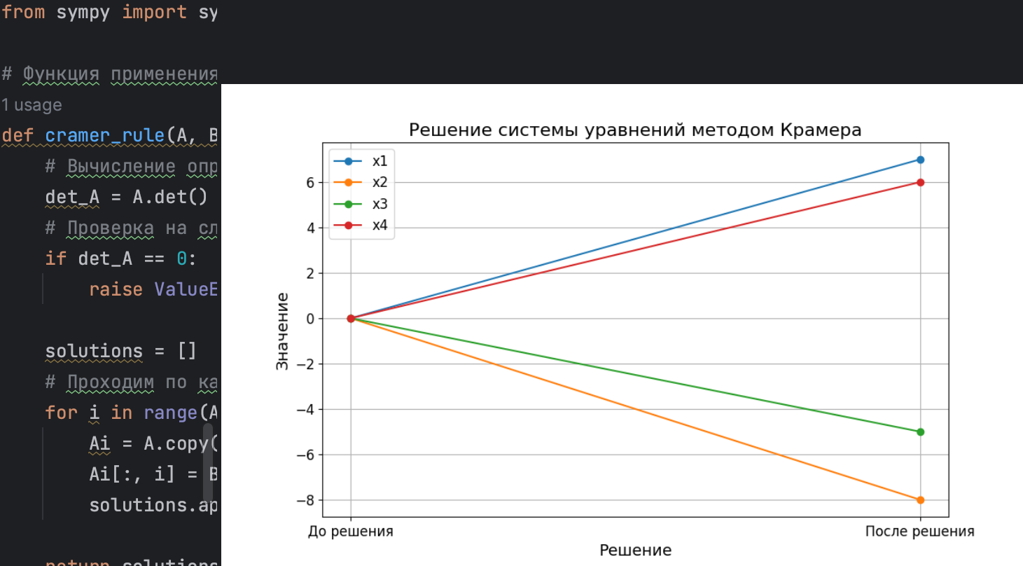
The code contains a function called cramer_rule, designed to apply Cramer's rule when solving systems of linear equations. It first calculates the determinant of the main matrix  then creates alternative matrices by replacing each of the matrix columns
  vector of constants
  calculating their determinants. Solutions of Variables
  are obtained by dividing the determinants of these alternative matrices by the determinant of the main matrix
  .
.
Then the code declares symbolic variables, as well as generates a matrix of coefficients  and column vector
  which is necessary to check the effectiveness of Cramer's rule.
Within the block try-except a function call is made cramer_ruleto find a solution to a system of equations using Cramer's method. In the case when the determinant of the main matrix is equal to zero, an exception is raised ValueError followed by displaying a corresponding message indicating that a solution cannot be solved. If the determinant is not equal to zero, the results, which are solutions of the system, are displayed on the screen.
Gauss method
The Gaussian method, also known as Gaussian elimination or stepwise transformation of a system of equations, is one of the fundamental approaches to solving systems of linear equations. This method involves performing elementary operations on the rows of a matrix of equations to transform it into a stepwise or simplified stepwise form, which greatly facilitates finding solutions to the system.
from sympy import Matrix, pprint


def print_row_reduced_matrix(matrix):
    print("Ступенчатая матрица:")
    pprint(matrix)


# Определение расширенной матрицы [A|B]
augmented_matrix = Matrix([
    [1, 1, 1, 1, 0],
    [5, -3, 2, -8, 1],
    [3, 5, 1, 4, 0],
    [4, 2, 3, 1, 3]
])

# Выполнение приведения матрицы к ступенчатому виду
row_reduced_matrix, _ = augmented_matrix.rref()

# Вызов функции для вывода ступенчатой матрицы
print_row_reduced_matrix(row_reduced_matrix)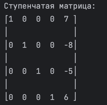
In the presented code, we start by defining an extended matrix, where the last column contains the free terms of the system of equations. Next, using the method .rref()which is provided by the object Matrix SymPy library, transform this matrix to echelon form.
After the transformation, the step matrix is displayed on the screen using the function print_row_reduced_matrixwhich allows you to visually evaluate changes in the structure of the matrix after applying the Gaussian method and determine the leading elements.
Numerical solution
Numerical solution of a system of equations is the process of determining approximate values of variables when an exact analytical solution is unattainable or undesirable. This approach is often used in situations where it is necessary to obtain a numerical approximation to solve a system.
from sympy import symbols, Eq, nsolve

# Определение переменных
x1, x2, x3, x4 = symbols('x1 x2 x3 x4')

# Определение системы уравнений
equations = [
    Eq(x1 + x2 + x3 + x4, 0),
    Eq(5*x1 - 3*x2 + 2*x3 - 8*x4, 1),
    Eq(3*x1 + 5*x2 + x3 + 4*x4, 0),
    Eq(4*x1 + 2*x2 + 3*x3 + x4, 3)
]

# Начальное предположение для численного решения
initial_guess = [0, 0, 0, 0]

# Нахождение численного решения
numerical_solution = nsolve(equations, (x1, x2, x3, x4), initial_guess)

# Вывод результатов
print("Численное решение:")
print(f"x1 = {numerical_solution[0]}")
print(f"x2 = {numerical_solution[1]}")
print(f"x3 = {numerical_solution[2]}")
print(f"x4 = {numerical_solution[3]}")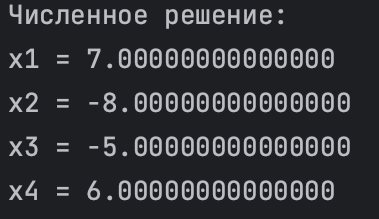
The code we're looking at uses the function nsolve from the SymPy library to determine the numerical solution to a set of equations. First the variables are defined x1, x2, x3 и x4 like symbols. Next, the system of equations is represented by a list of instances Eq. Then the initial approximation for the solution is indicated, represented by the list initial_guess.
Function nsolve requires a list of equations as input (equations), list of symbolic variables (x1, x2, x3, x4) and initial approximation (initial_guess). It calculates a numerical approximation of the values of the variables that is as close as possible to the analytical solution, and returns the resulting values in list form.
Each found numerical value of the variables x1, x2, x3 и x4 is displayed as a separate line.
Least square method
Least squares is a statistical procedure used to make an optimal fit to data. It consists of finding a function that minimizes the total sum of squares of the difference between the actual values and the values predicted by the model. This method is especially useful when working with overdetermined systems of linear equations, that is, when the number of equations exceeds the number of unknowns.
from sympy import symbols, Matrix

# Определение переменных
variables = symbols('x1 x2 x3 x4')

# Определение матрицы коэффициентов
coefficients_matrix = Matrix([
    [1, 1, 1, 1],
    [5, -3, 2, -8],
    [3, 5, 1, 4],
    [4, 2, 3, 1]
])

# Определение матрицы значений
constants_matrix = Matrix([0, 1, 0, 3])

# Решение системы с помощью метода наименьших квадратов
least_squares_solution = coefficients_matrix.solve_least_squares(constants_matrix)

# Вывод решения
print("Решение методом наименьших квадратов:", least_squares_solution)
Here we use the function solve_least_squares from the object Matrix SymPy libraries for solving systems of linear equations with excess conditions using the least squares method. Variables are entered first x1, x2, x3 и x4. Then matrices are created: one for the coefficients (coefficients_matrix) and one for free members (constants_matrix) systems of equations.
Function solve_least_squares takes these two matrices and finds a decision vector that minimizes the sum of squared differences between the product of the coefficient matrix and the decision vector and the real data contained in the dummy term matrix.
Symbolic solution
Symbolic solving of a system of equations is an approach in which variables are treated as symbols and mathematical algorithms are applied to obtain their exact analytical values. Unlike numerical methods, in which the values of variables are found numerically, the symbolic solution produces formulas for the variables, possibly including other symbols.
from sympy import symbols, Eq, solve

# Определение переменных
x1, x2, x3, x4 = symbols('x1 x2 x3 x4')

# Определение системы уравнений
equations = [
    Eq(x1 + x2 + x3 + x4, 0),
    Eq(5*x1 - 3*x2 + 2*x3 - 8*x4, 1),
    Eq(3*x1 + 5*x2 + x3 + 4*x4, 0),
    Eq(4*x1 + 2*x2 + 3*x3 + x4, 3)
]

# Решение системы символьно
symbolic_solution = solve(equations, (x1, x2, x3, x4))

# Вывод решения
print("Символьное решение:", symbolic_solution)

The demonstrated code starts by defining symbolic variables x1, x2, x3 и x4after which the system equations are formed into a collection of objects Eq. To solve the system symbolically, use the function solve from the SymPy library. This function receives a list of equations as input (equations) and a list of corresponding symbolic variables (x1, x2, x3, x4), and returns a dictionary with analytical solutions for each of the variables.
In this article, we looked at one of the functions of the SymPy library: solving systems of linear equations using different methods, the choice of which is determined by specific tasks.
From a student's perspective, it is not just knowledge of these techniques that is important, but a deep understanding and ability to apply them in practice is important, as this can provide valuable experience in many areas of science and engineering.
The choice of the SymPy library for this review was not accidental: it allows you to perform symbolic calculations, processing expressions as a series of symbols, which significantly increases the accuracy of mathematical operations. In addition, the library covers a variety of areas of mathematics, including solving equations and working with matrices. An added benefit is its compatibility with other tools, such as the Matplotlib library, making SymPy easy to integrate to expand its capabilities.
Thanks for reading)