How organ cell growth is investigated using physics-based machine learning
… as well as deep learning based on cloud computing and acoustic modeling
To grow organ tissue from cells in the laboratory, researchers need a non-invasive way to keep cells in one place. One promising approach is acoustic structuring, which involves the use of acoustic energy to position and hold cells in a desired position as they develop in tissue. By applying acoustic waves to microfluidic devices, the researchers turned micron-scale cells into simple patterns such as straight lines and gratings.
My colleagues and I have developed a combined approach to deep learning and numerical modeling that allows us to arrange cells into much more complex circuits of our own architecture. We saved weeks of effort by doing the entire workflow in MATLAB and using parallel computing to speed up key steps such as generating the training dataset from our simulator and training the deep learning neural network.
Acoustic modeling with microchannels
In a microfluidic device, fluid particles and fluid-borne particles or cells are driven in sub-millimeter-sized microchannels, which can be configured in various shapes. To create acoustic patterns within these microchannels, an interdigital transducer (IDT) generates a surface acoustic wave (SAW) directed towards the channel wall (Fig.1a). In the liquid inside the channel, acoustic waves create a minimum and maximum pressure, which is equal to the pressure of the channel wall (Fig. 1b). Therefore, the shape of the channel walls can be adjusted in such a way that it would give certain acoustic fields in the channel. [1] (Fig. 1c). The acoustic fields distribute particles within the fluid in patterns that correspond to the locations where the forces from these acoustic waves are minimized (Figure 1d).
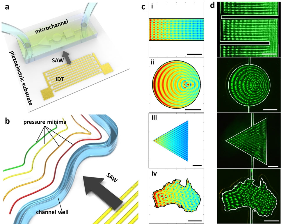
Figure 1 – Acoustic structuring in microchannels
While it is possible to compute the acoustic field that will result from a particular canal shape, the opposite is not possible: designing the canal shape to create the desired area is not a trivial task for anything but simple mesh-like patterns. Since the solution space is virtually unlimited, analytical approaches are inapplicable.
The new workflow uses a large collection of simulated results (randomized forms) and deep learning to overcome this limitation. My colleagues and I solved a direct problem for the first time by simulating pressure fields from known shapes in MATLAB. We then used the results to train a deep neural network to solve the inverse problem: determining the shape of the microchannel needed to create the desired acoustic field.
Solving the Direct Problem: Modeling Pressure Fields
In previous work, our team developed a simulation engine in MATLAB that solves the problem of determining the pressure region for a given channel geometry using the Huygens-Fresnel principle, which assumes that any point on a plane wave is a point source of spherical waves (Fig. 2).
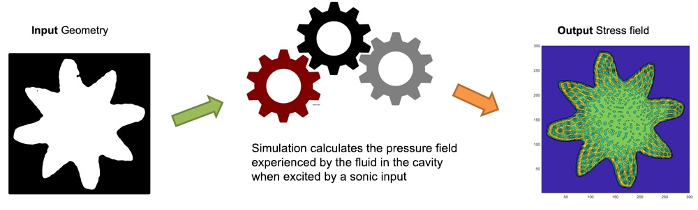
Figure 2 – The acoustic pressure field created for a certain geometry of the channel
The simulation engine relies on various matrix operations. Since these operations are performed in MATLAB, each simulation takes a fraction of a second, and we needed to simulate tens of thousands of unique shapes and their corresponding 2D pressure regions. We accelerated this process by running simulations in parallel on a multi-core workstation using Parallel Computing Toolbox.
Once we had the data we needed, it was used to train the deep learning network to infer the shape of the channel from a given pressure area, essentially reversing the order of input and output.
Train deep learning neural network to solve inverse problem
First, to accelerate the training process, a threshold value was determined on the simulated pressure area. As a result, two-dimensional boolean matrices 151 x 151 were created, which we transformed (“flattened”) into a one-dimensional vector, in turn, it would become an input to the deep learning network. To minimize the number of output neurons, we used the representation of the Fourier coefficient, which captured the contour of the channel shape (Fig. 3).

Figure 3 – Approximation of the Fourier series of an equilateral triangle rotated by 20 degrees with coefficients (from left to right) 20, 3, 10 and 20
We built the original network using the Deep Network Designer and programmatically enhanced it to balance accuracy, versatility, and learning speed (Figure 4). We trained the network using an adaptive torque estimation solver (ADAM optimizer) on an NVIDIA Titan RTX GPU.
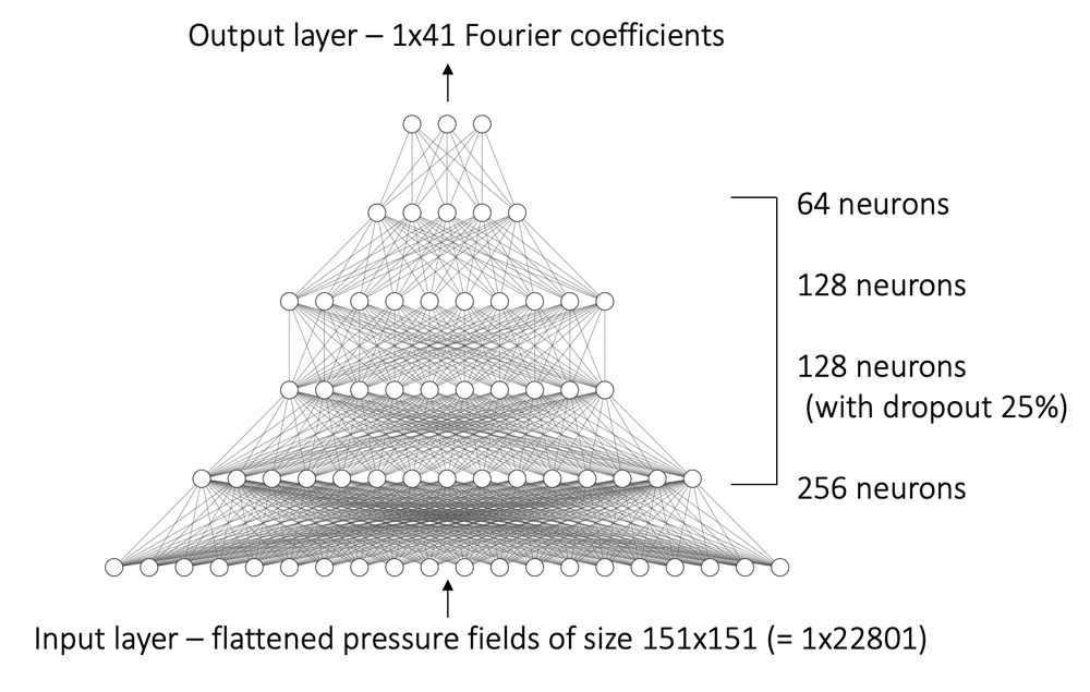
Figure 4 – Fully connected neural network with four hidden layers
Checking results
To validate the trained network, we used it to derive the channel geometry from a given pressure field, and then used that geometry as input to the simulation engine to reconstruct the pressure field. We then compared the original and created pressure fields. The minimum and maximum pressures within the two fields are close to each other (Fig. 5).
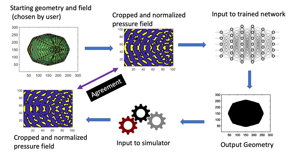
Figure 5 – Deep learning network validation workflow
Then we ran a series of real tests. To indicate the areas where we wanted to collect the particles, we painted specialized images using Microsoft Paint. They contained many different single and multiline images that would be difficult to obtain without our method. The trained network was then used to define the geometry of the channels needed to create these defined areas. Finally, with the help of our partners, we have manufactured a range of microfluidic devices based on the intended geometry. Each of these devices was then injected with 1 μm polystyrene particles suspended in a liquid into the formed channels, and a surfactant was induced on the device. The results showed particle aggregation along the regions that were indicated in our specialized images (Fig. 6).

Figure 6 – Bottom: Areas drawn in Microsoft Paint (purple) are superimposed on the simulated acoustic field required for particle aggregation in these areas; top: the result is a sample of suspended polystyrene particles in a manufactured microfluidic device
Going to the cloud
In anticipation of the next phase of this project, we are updating our deep learning network to use acoustic field images as inputs and generate channel shape images as outputs, rather than using squished vector and Fourier coefficients, respectively. The hope is that this change will allow us to use channel shapes that are not easy to determine with the Fourier series and that can change over time. However, training will require a much larger dataset, a more complex network architecture, and significantly more computational resources. As a result, we transfer the network and its training data to the cloud.
Fortunately, MathWorks Cloud Center provides a convenient platform for quickly spinning up and out of HPC cloud instances. One of the more tedious aspects of doing scientific research in the cloud is interoperability, which involves moving our algorithms and data between the cloud and our local machine. MATLAB Parallel Server abstracts the more complex aspects of cloud computing by allowing us to run locally or in the cloud with a few simple menu clicks. This ease of use allows us to focus on the scientific problem rather than the tools needed to solve it.
Using MATLAB with NVIDIA GPU-powered Amazon Web Services instances, we plan to train the updated network on data stored in Amazon S3 buckets. We can then use the trained network on local workstations to draw conclusions (which do not require high performance computing) and experiment with different patterns and acoustic fields. This work will provide us with the raw data for other machine learning projects using physics.
If you want to know more about machine and deep learning – check out our corresponding course, it will not be easy, but exciting. A promo code HABR – will help in the desire to learn new things by adding 10% to the discount on the banner.

- Machine Learning Course
- Advanced Course “Machine Learning Pro + Deep Learning”
- Data Science profession training
- Data Analyst training
- Java developer profession
- Frontend developer profession
- Profession Ethical hacker
- C ++ developer profession
- Profession Unity Game Developer
- The profession of iOS developer from scratch
- Profession Android developer from scratch
- Profession Web developer
COURSES
- Python for Web Development Course
- JavaScript course
- Course “Mathematics and Machine Learning for Data Science”
- Data Analytics Course
- DevOps course