Development of a servo drive with a BLDC motor

The open source project of the MC50 servo controller continues to evolve. This time we will talk about creating a servo.

Servo drives are needed everywhere in a smart home: in stopcocks, in electric locks, in motorized brackets, tables, blinds, in automatic doors, gates, windows, awnings, gates, PTZ cameras, adjustable chairs, electric ramps, and so on. Therefore, servo technology is in high demand and there is room for creativity.

Previous articles related to the MC50 project

In the last article, it was shown how to make a BLDC motor spin using the peripherals of the S5D9 microcontroller of the Renesas Synergy ™ family.

Now this rotation must be made to do useful work. Outside observers can tell that the work has already been done if the motor is rotating, the goal is achieved. Put the gearbox and in prod. But in fact, the problems are just beginning.

Design

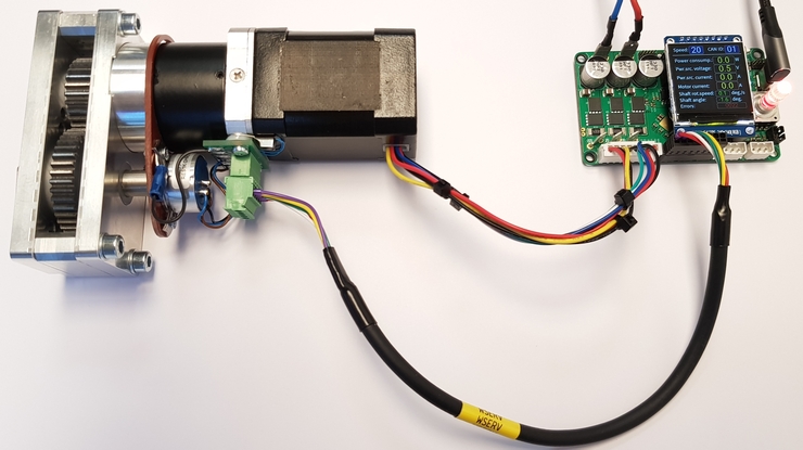
The design consists of a gear motor, an additional 29/40 gear, a simple assembly with a servo potentiometer to control the speed of the output shaft and a thermistor to control the temperature of the motor. As you can see, the external gearbox makes it convenient to place the servo potentiometer. In addition, it increases the moment of force by 1.3 times. Such a design in various scales is found in many servos.

Wiring diagram

The servo controller board is designed to be powered from an external source with a voltage of 20 to 30 V. But the power driver continues to function when the voltage drops to 7 V. If there is no external voltage source, the board can be powered from USB, but the power driver will not function.

About the speed of the BLDC motor

The rotational speed of a BLDC motor is determined by the voltage applied to it under the condition of a constant load on the shaft (we assume that the 6-step switching works flawlessly at this time, we change the voltage with PWM). This frequency is recorded in the datasheet on the motor. If the moment of the load force is greater or less, then the frequency will be different at a constant voltage. But we do not know exactly the moment of the load force and it is likely to be variable.

For an ideal motor with no load, no friction and no winding resistance, the rotational speed at a certain voltage can be found by rotating the motor with an external drive until the specified voltage is reached. The rotational speed at this moment will be the desired frequency. But here the form of tension is important. Applying 6-step commutation to a motor with sinusoidal back EMF will not get the same frequency.

An ideal BLDC motor will spin at infinite speed when an infinite voltage is applied to it. In a real BLDC engine, at some point, the magnetic circuit will first saturate, the current through the windings will increase sharply, the windings will heat up and after a while the motor will light up. Therefore, the speed and the permissible moment of force are still limited by the temperature of the motor.

Development of management architecture.

If the architecture is clear enough for controlling a bare motor, then for controlling a servo drive with unknown load dynamics, everything is somewhat more complicated.

To begin with, we note that the rotor speed is not equal to the servo speed, and in dynamics with real mechanics with backlash and elastic reactions, it is not even proportional.

For speed control, the easiest solution is to simply change the pulse width modulation (PWM) duty cycle.

Model file here

With a constant load torque on the motor or manual control, everything works out pretty well. We linearly change the duty cycle and achieve the desired speed. Switching is automatic with Hall sensors located in the motor. The method works great in scooters

But as soon as the moment of force begins to change, the rotation frequency will begin to pulsate, as shown in the video below.

The most obvious solution is to use PID control with speed feedback. Unfortunately, everything is not so simple. Servo drives can be designed for angular velocity control or for position control, in both cases different algorithms are needed. And in both cases, a simple single-loop PID performs very poorly. In the case of position stabilization, a regulator with a transient response of at least the third order is needed. And PID has the second order. Those. staying within the PID requires two control loops nested one inside the other. We need a good, fast, optimizable, scalable implementation of the PID algorithm.

Such an implementation is available in the MATLAB Simulink environment in the form of a model converted to C source code. Below is a model in the form of an open extensible subsystem.

Model files are here.

The model replicates the functionality of the built-in Simulink PID component, but outputs all PID coefficients as input arguments on a single bus. Arguments can also be changed in a standard component using variable symbols from the workspace, but this entails implicit dependencies leading to errors. And the bus provides the generation of the argument as a transferable structure. This reduces the amount of code when integrating a model into an embedded project and simplifies model refactoring.

To prevent the infinite growth of the integral component (anti-windup), the clamping method is applied.

In addition, our model implements a slew rate limiter. This adds additional protection to the model from limiting oscillations in case of using incorrect initial coefficients during tuning.

The sources generated from the model are located in the directory MATLAB_PID.

Choice of single loop or dual loop servo speed control.

To make a choice of control loop architecture, let’s conduct an experiment. Let’s make two recordings of signals in the FreeMaster environment in different motor control modes. We will record four signals simultaneously:

• turn-on signal

• current flowing through the motor

• the status of the Hall sensors, reflecting the speed of rotation of the rotor

• drive output speed.

The first recording below is made during a 6-step motor hopping at maximum voltage.

The second recording below is made during 6-step motor hopping with constant current through the motor using the current control loop.

If you look at the response of the speed of the output shaft to the jump in action, then the first record shows an extremely non-linear speed curve. On the second record, the speed increases quite linearly, but the increase starts with some delay.

Obviously, in the first case, it will be practically difficult to adjust the speed by adjusting the PWM duty cycle using the PID algorithm. In any case, with a control interval of less than 0.1 sec. Because speed responds in a completely different way than a linear system. And the classic PID is only good for linear systems.

In the second case, the response is much more linear and the PID is fine here. Rather, a simple PI circuit will do here, since the response shows an inertial load without elasticity (oscillations). But we must remember – a high-speed circuit for supporting a given current has already been applied here. Those. in this case we have a 2-loop system: a fast PI loop to control current via PWM and a slow PI loop to control speed via current reference.

As a result, we came to the following architecture as part of the Simulink model:

Model file here

The model includes a gear motor with planetary gear and Hall sensors, an external gearbox, a servo sensor with a speed measurement model including measurement noise, a 3-phase inverter with CMOS transistors, a PWM modulator and two control loops: speed and current. The colors on the model highlight areas that work with different clock rates. The current loop operates at a frequency of 16 kHz, the speed loop at a frequency of 100 Hz.

Measurement of rotor speed with Hall sensors

In the model shown above, the rotor speed is measured by Hall sensors. But in reality, it turned out that measuring the duration of the intervals between the pulse fronts from the sensors is poorly suited for determining the rotor speed. From the graph below it follows that at a constant frequency, the difference in the duration of the intervals can be up to 30%. Such an error will then be expressed in insufficient accuracy or speed of stabilization of the rotational speed.

In our program, we use a different way of measuring rotational speed. The timers capture the time of each signal edge, but the difference is not counted from the previous edge, but from the last edge of the same pole.

The logic for capturing the GPT3211 and GPT3212 timers is used (according to the header from the SSP, they are named R_GPTB3 and R_GPTB4). The timers have two capture modules, so two timers are needed for signals from three sensors. Timers are clocked absolutely synchronously thanks to the simultaneous start command (all timers in Synergy can be started synchronously).

Here’s a snippet how the measurement is made in the interrupt handler from the ADC:

  st = R_GPTB3->GTST;  // Читаем флаги состояния capture таймера  GPT3211

  if (st & BIT(0))     // Проверяем флаг TCFA. Input Capture/Compare Match Flag A
  {
    // Здесь если событие захвата произошло

    R_GPTB3->GTST = 0;      // Очищаем флаг захвата и остальные флаги.
                            // За другие флаги захвата не беспокоимся, поскольку они при штатной работе не могут быть взведены в этот момент.

    val = R_GPTB3->GTCCRA;  // Читаем регистр с захваченным состоянием счетчика

    // Здесь рассчитываем разницу по отношению к предыдущему захваченному значению на том же угле поворота ротора, т.е. для полюса с номером в переменной hall_u_cnt
    if (hall_u_prev_arr[hall_u_cnt] > 0)
    {
      if (val > hall_u_prev_arr[hall_u_cnt])
      {
        hall_u_capt_arr[hall_u_cnt] = val - hall_u_prev_arr[hall_u_cnt];
      }
      else
      {
        // Корректируем если было произошло переполнение счетчика между захватами
        hall_u_capt_arr[hall_u_cnt] =  0x7FFFFFFF -(hall_u_prev_arr[hall_u_cnt] - val -1);
      }

      hall_u_capt = hall_u_capt_arr[hall_u_cnt]; // Сохраняем разницу в промежуточную переменную. Эта переменная используется при отладке через FreeMaster
      // .......................................................
      one_turn_period = hall_u_capt;             // Записываем длительность полного оборота ротора в глобальную переменную для дальнейшего использования остальными задачами
      // .......................................................
    }
    hall_u_prev_arr[hall_u_cnt] = val;         // Сохраняем текущее захваченное значение в переменную предыдущего значения
    hall_u_cnt++;                              // Ведем счет полюсов. Для каждого полюса сохраняется своя измеренная величина
    if (hall_u_cnt >= 8) hall_u_cnt = 0;

    // Определяем направление вращения
    h = R_IOPORT5->PCNTR2 & 0x7;  // Читаем сигналы датчиков Холла здесь снова, несмотря на то что они уже были прочитаны в обработчике прерывания
                                  // Это нужно поскольку capture логика может сработать уже после того как в ISR были прочитаны состояния датчиков
    if ((h == 0b100) || (h == 0b011))      rotating_direction = 1; // Направление вращения определяем по паттернам сигнало с датчиков сразу после текущего фронта
    else if ((h == 0b010) || (h == 0b101)) rotating_direction = -1;

    R_GPTB5->GTCLR_b.CCLR13 = 1;  // Сброс счетчика отслеживающего остановку вращения
    R_GPTB5->GTST           = 0;  // Сброс флагов счетчика отслеживающего остановку вращения
  }

  if (st & BIT(1))
  {
    // Input capture/compare match of GTCCRB occurred
    R_GPTB3->GTST = 0;
    val = R_GPTB3->GTCCRB;
    if (hall_v_prev_arr[hall_v_cnt]>0)
    {
      if (val > hall_v_prev_arr[hall_v_cnt])
      {
        hall_v_capt_arr[hall_v_cnt] = val - hall_v_prev_arr[hall_v_cnt];
      }
      else
      {
        hall_v_capt_arr[hall_v_cnt] =  0x7FFFFFFF -(hall_v_prev_arr[hall_v_cnt] - val -1);
      }
      hall_v_capt = hall_v_capt_arr[hall_v_cnt];
      one_turn_period = hall_v_capt;
    }
    hall_v_prev_arr[hall_v_cnt] = val;
    hall_v_cnt++;
    if (hall_v_cnt >= 8) hall_v_cnt = 0;

    h = R_IOPORT5->PCNTR2 & 0x7;  // Читаем сигналы датчиков Холла здесь чтобы они были прочитаны не раньше чем стработает capture логика
    if ((h == 0b110) || (h == 0b001))      rotating_direction = 1;
    else if ((h == 0b011) || (h == 0b100)) rotating_direction = -1;

    R_GPTB5->GTCLR_b.CCLR13 = 1;  // Сброс счетчика отслеживающего остановку вращения
    R_GPTB5->GTST           = 0;
  }


  st = R_GPTB4->GTST;

  if (st & BIT(0))
  {
    // Input capture/compare match of GTCCRA occurred
    R_GPTB4->GTST = 0;
    val = R_GPTB4->GTCCRA;
    if (hall_w_prev_arr[hall_w_cnt]>0)
    {
      if (val > hall_w_prev_arr[hall_w_cnt])
      {
        hall_w_capt_arr[hall_w_cnt] = val - hall_w_prev_arr[hall_w_cnt];
      }
      else
      {
        hall_w_capt_arr[hall_w_cnt] =  0x7FFFFFFF -(hall_w_prev_arr[hall_w_cnt] - val -1);
      }
      hall_w_capt = hall_w_capt_arr[hall_w_cnt];
      one_turn_period = hall_w_capt;
    }
    hall_w_prev_arr[hall_w_cnt] = val;
    hall_w_cnt++;
    if (hall_w_cnt >= 8) hall_w_cnt = 0;

    h = R_IOPORT5->PCNTR2 & 0x7;  // Читаем сигналы датчиков Холла здесь чтобы они были прочитаны не раньше чем стработает capture логика
    if ((h == 0b101) || (h == 0b010))      rotating_direction = 1;
    else if ((h == 0b110) || (h == 0b001)) rotating_direction = -1;

    R_GPTB5->GTCLR_b.CCLR13 = 1;  // Сброс счетчика отслеживающего остановку вращения
    R_GPTB5->GTST           = 0;
  }

Here we get the value of the rotation frequency with a deviation of less than 0.3%, but with a much greater delay than we could get by measuring the durations between adjacent fronts. But in the latter case, we would have to apply a filter that would introduce even more delay.

Speed ​​extrapolation at sudden stop

The rotation of the rotor may suddenly stop when the servo encounters an obstacle. But then the block for calculating the rotational speed using Hall sensors will simply not be executed. As a result, the frequency readings will freeze, and the 6-step switching algorithm will freeze on the constant inclusion of one branch of the winding. Therefore, it is necessary to implement a block for extrapolating the rotational speed in the absence of signals from the Hall sensors. An example implementation is shown below.

  // Блок линейно понижающий скорость в случает отсутствия сигналов с датчиков Холла
  if (one_turn_period != 0)
  {
    if (R_GPTB5->GTST & BIT(6))  // Проверяем флаг TCFPO. Overflow Flag
    {
      // В случае переполения тамера сразу отмечаем скорость как нулевую.
      // Поскольку переполение таймера происходит с периодом в две секунды, то такую низкую скрость принимаем как нулевую
      one_turn_period = 0;
    }
    else
    {
      // За один оброт мотора мы имеем 8 полюсов * 3 датчика = 24 события сброса таймера R_GPTB5
      // И если таймер R_GPTB5 смог набрать 2/3 (16/24) длительности одного оборота и не был сброшен значит скорость упала
      // и можно начинать снижать оценку текущей скорости
      uint32_t no_edge_period = R_GPTB5->GTCNT*16;
      if (no_edge_period > one_turn_period)
      {
        one_turn_period = no_edge_period;
      }
    }
  }

After some time, the speed indicator will drop to zero and the speed control algorithm will decide to turn off the current.

Influence of the switching method of power transistors on the quality of control and power consumption

In a previous article about 6-step switching control several ways of switching transistors during PWM modulation have been shown. There are two ways in our program. You can choose between them by setting the Enable soft communication parameter.

On our gearmotor, these two methods showed only minor differences. At the same rotational speed, the current consumption was identical. But with soft switching, the rotation of the motor began at a lower duty cycle. The fact is that the motor, due to friction, does not start spinning until the PWM duty cycle exceeds a certain threshold. This threshold in the case of hard switching in our case was in the region of 55%, and in the case of soft switching, in the region of 30%. Those. soft switching gives a larger PWM control range – 70%, as opposed to hard switching – 45%. This is then reflected in the quality of speed control. With soft switching, the quality of control is somewhat better.

The switching method is selected by the parameter en_soft_commutation.

Adjusting the gate current of power transistors

The servo controller board uses the TMC6200 driver chip. The microcircuit receives signals from the microcontroller and controls the gates of power transistors. The microcontroller cannot directly drive the gates because they need high voltages and rather large pulse currents.

This microcircuit has the ability to set the level of output currents to the gates via the SPI interface. There are 4 levels: from the weakest 400…600 mA to the strongest 1200…1800 mA.

As tests of all possible levels have shown, they practically do not affect the current consumption. Power measurements during engine operation are very noisy, and given this noise, it is possible to assume that there is some difference within 100 mW.

The power transistors in the circuit are optimally matched to the driver, so adjusting its strength does not have a noticeable effect. It is to be expected in the general case that the greater the driver current, the greater the losses in it. In the program settings, you can freely change the levels of currents, as well as the levels of detection and protection against short circuits.

You can manage the TMC6200 driver settings with using a number of parameters. Settings are loading at the start of the main motor control task.

Offset Calibration of TMC6200 Driver Current Amplifiers

The TMC6200 chip has built-in voltage amplifiers with current shunts located in the servo driver phases. The presence of built-in amplifiers simplifies the circuit. It is possible to change the gain through the SPI interface.

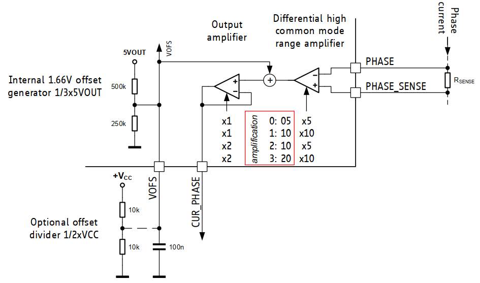
However, the disadvantage of these amplifiers is the rather high bias voltage. Even worse, it is highly dependent on the temperature of the chip. But not only that, it is different for each of the 3 amplifiers and can change over time even at a constant external temperature. Our program uses the most sensitive mode with a 20x gain. With this gain, the bias at the output of the amplifiers reaches 240 mV or more.

The solution to the problem is found in the fact that before each engine is turned on, offset zero recalibrationI for each of the 3 amplifiers. Recalibration lasts about 15 ms and has no significant effect on performance.

What to do with back EMF?

As soon as the motor starts to turn external forces instead of our driver, it turns into a generator. The motor also turns into a generator for short periods of time when braking occurs. If the speed caused by external forces exceeds the speed at rated voltage at no load, then the voltage on the power rail increases. The waveform below shows the voltage spikes on the power rail when the servo rotates the weight on the arm at a constant PWM value. At the moments when the load is lowered, the voltage on the power bus rises by 5.5 V. This is because the rotor speed at these moments exceeds the maximum speed at the rated voltage according to the datasheet.

If we controlled the speed and did not allow the servo to accelerate, then there would be no such voltage surges. However, power surges can also occur when the servo is off. Then this is the strategy. When the voltage reaches a level sufficient to turn on the processor, it immediately sends a turn-on signal to all lower transistors. The transistors short the motor windings and the voltage drops.

The problem of determining the speed of rotation of the servo potentiometer

If you look closely at the signal coming from the servo-potentiometer mounted on the output shaft, you will notice that it contains quite a significant amount of noise.
To find the speed, you need to get the function of the differential of the angle of rotation from time. With digital control, this will simply be the difference between the current position and the previous position. As can be seen from the screenshot, after such an operation, an absolutely noisy signal is obtained. In this case, we apply deep two-stage filtration. Filtering is performed with a PWM frequency i.e. 16 kHz

Since the filter introduces a phase delay, we cannot control arbitrarily quickly and accurately based on such a filtered signal.

You need to find out the frequency at which the phase at the output of the filter will become inverse with respect to the phase at the input. To do this, we construct an auxiliary model for testing our heuristic filter

Here we do not resort to complex analyzers and equalizers, but simply look at the order of transitions through zero. As soon as the sequence is violated, then there is a strong phase shift between the compared signals.

At the time point 11.4 sec we see the first anomaly. This will be the site of the first phase inversion. It is easy to understand that the frequency at this point will be equal to 1140 Hz. Therefore, after our filter, we cannot speed up the PID controller faster than 1000 times per second, otherwise excitation may occur in the control loop. Increasing the length of the running average filter by a factor of two also reduces the limiting control frequency by a factor of two.

Application development for MC50

Software framework servo controller MC50 is based on Azure RTOS. At this stage, it contains almost the entire composition of the Azure RTOS middleware with peripheral drivers. On top of the middleware layer is several applied tasks: motor control, 3-phase motor driver chip control, measurement, GUI, output control and others.

The current version of the software implements lever control at specified angles at a specified speed. The hand encoder is used to calibrate the angles, adjust the rate of turn and set the node number on the CAN bus. All other parameters can be configured via terminal VT100 via USB VCOM or via the Internet, as shown in previous articles. Servo commands can be given with manual encoderBy CAN bus and through protocol free master via USB.

Development continues…