Coefficients for extrapolating 5-year CLTV component forecasts
This article describes how to derive customer value over a 5-year horizon from predictions from a number of ML models. Let us recall that the CLTV indicator is a composition of forecasts of its components (more details in the article). In our implementation, the maximum model forecasting period is 24 months. It is important to note that the higher the forecast horizon, the less accurate the model can make a forecast. And the CLTV indicator is interesting for business over a longer horizon, in our case – five years. How can you get a five-year forecast from two-year forecasts? The answer is simple: extrapolate forecasts.
The main idea of extending (extrapolating) forecasts is to divide users into several groups, and in each group to uniformly extend the forecast series.
Next we will discuss:
approaches to series extrapolation, their advantages and problems
how to select groups and prepare data for extrapolation
advantages of the chosen approach to extending forecasts for 5 years, difficulties and ways to solve them.
1. Approaches to extrapolation
So, let's figure out what we need to extrapolate and how we can do it. We have access to monthly forecasts for each of the CLTV components for 24 months. The final goal is to derive some coefficients with the help of which, having a forecast for 24 months, we can obtain a forecast for 25, 26, 27, … 60 months. To do this, it is necessary to extrapolate or extend a number of forecasts.
To construct coefficients, we have access to historical and forecast data.
In our opinion, calculating coefficients based on historical data (facts) has many disadvantages, since their changes are influenced by many external factors (changes in the cost of tariff plans, crises, actions of competitors), the influence of which we want to avoid and study separately through experiments and tests. In addition, for 5-year extrapolation coefficients it would be necessary to use very old historical data, which would lead to out-of-date coefficient values. For example, subscriber behavior (in particular, survival rate) in the last year is different from their behavior 3 years ago. For the same reason, ML models do not predict revenue and costs over a 5-year horizon. The advantages of this approach include the availability of information about actual fluctuations in the service margin over long horizons. As a result of this approach, if the basis improves every year, we will obtain underestimated coefficient estimates. We used historical data only for validation.
For the reasons described above, predicted values were used to construct the coefficients. For extrapolation, we built regressions with more or less monotonically decreasing/increasing series of forecasts. However, it is not always possible to see such a dependence in a series of data; in this case, you can look at a series of forecasts calculated with a cumulative total and thus arrive at monotonicity.
Example: there are a number of observations over 2 years for a user base active in December 2021 (a group of users was recorded). Observation = the amount of revenue we forecast for 1, 2, 3… 24 months ahead. We will depict the described series with a blue line on the graph, where the x-axis is the month of the forecast, and the y-axis is revenue. We see that the blue line first decreases and then fluctuates around zero. Orange shows the series calculated as a cumulative total – it shows a clear logarithmic relationship between the accumulated revenue forecast and the month of the forecast.
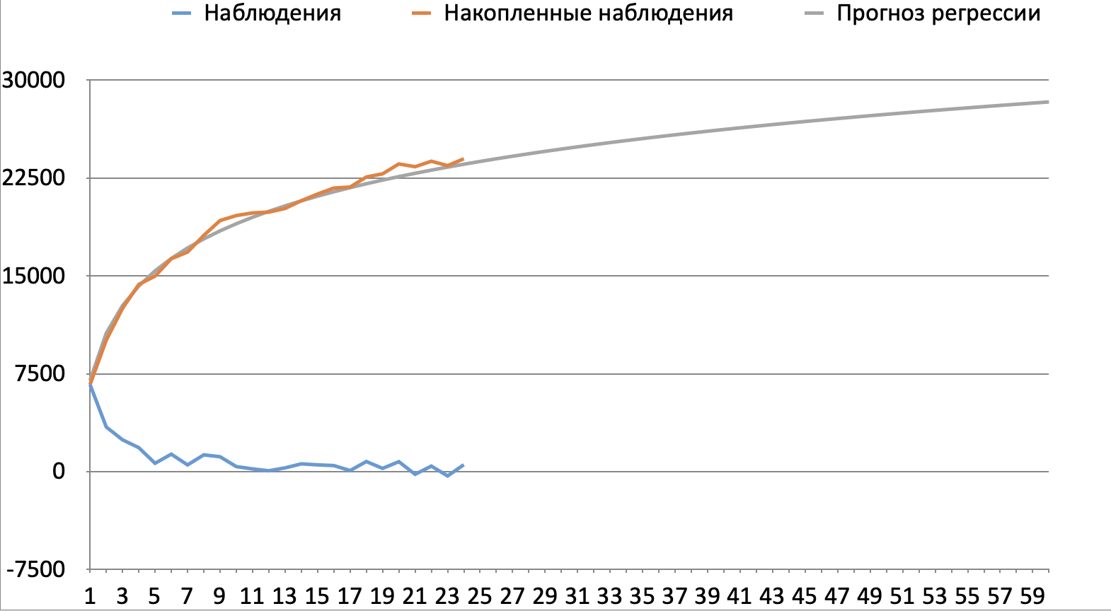
Data for the graph
Margin fact | Accumulated fact | Forecast | period | |
2020-01-01 | 6666 | 6666 | 7000 | 1 |
2020-02-01 | 4199.3599479678 | 10865.3599479678 | 10612.3599479678 | 2 |
2020-03-01 | 2683.0951086681 | 13548.4550566359 | 12725.4550566359 | 3 |
2020-04-01 | 1245.2648392996 | 14793.7198959355 | 14224.7198959355 | 4 |
2020-05-01 | 1263.9201560967 | 16057.6400520322 | 15387.6400520322 | 5 |
2020-06-01 | 949.1749525715 | 17006.8150046037 | 16337.8150046037 | 6 |
2020-07-01 | 658.3614755674 | 17665,1764801711 | 17141,1764801711 | 7 |
2020-08-01 | 423.9033637322 | 18089.0798439033 | 17837.0798439033 | 8 |
2020-09-01 | 781.8302693686 | 18870.9101132719 | 18450.9101132719 | 9 |
2020-10-01 | 15.0898867281 | 18886 | 19000 | 10 |
2020-11-01 | 1090.7122218988 | 19976.7122218988 | 19496.7122218988 | eleven |
2020-12-01 | 619.4627306726 | 20596.1749525714 | 19950.1749525714 | 12 |
2021-01-01 | 784.1452751107 | 21380.3202276821 | 20367.3202276821 | 13 |
2021-02-01 | 547.2162004568 | 21927.5364281389 | 20753.5364281389 | 14 |
2021-03-01 | 221.5586805293 | 22149.0951086682 | 21113.0951086682 | 15 |
2021-04-01 | 194.3446832028 | 22343.439791871 | 21449.439791871 | 16 |
2021-05-01 | -22.0527353318 | 22321.3870565392 | 21765.3870565392 | 17 |
2021-06-01 | 582.8830047005 | 22904,2700612397 | 22063.2700612397 | 18 |
2021-07-01 | -275.2268498057 | 22629.043211434 | 22345.043211434 | 19 |
2021-08-01 | 131.3167365338 | 22760.3599479678 | 22612.3599479678 | 20 |
2021-09-01 | -318.7284111608 | 22441.631536807 | 22866.631536807 | 21 |
2021-10-01 | 426.4406330595 | 22868.0721698665 | 23109.0721698665 | 22 |
2021-11-01 | 21.6618623446 | 22889.7340322111 | 23340.7340322111 | 23 |
2021-12-01 | 389.8008683282 | 23279.5349005393 | 23562.5349005393 | 24 |
2022-01-01 | -77.2547964748 | 23202.2801040645 | 23775.2801040645 | 25 |
2022-02-01 | 605.4000715853 | 23807.6801756498 | 23979.6801756498 | 26 |
2022-03-01 | 517.6849942581 | 24325.3651699079 | 24176.3651699079 | 27 |
2022-04-01 | 513.5312061987 | 24838.8963761066 | 24365.8963761066 | 28 |
2022-05-01 | 82.8795986809 | 24921.7759747875 | 24548.7759747875 | 29 |
2022-06-01 | 572.6790818484 | 25494.4550566359 | 24725.4550566359 | thirty |
2022-07-01 | 657.8852693753 | 26152.3403260112 | 24896.3403260112 | 31 |
2022-08-01 | -7.5405861723 | 26144.7997398389 | 25061.7997398389 | 32 |
2022-09-01 | -77.6324613042 | 26067,1672785347 | 25222.1672785347 | 33 |
2022-10-01 | 92.5797259724 | 26159.7470045071 | 25377.7470045071 | 34 |
2022-11-01 | 693.0695276963 | 26852.8165322034 | 25528.8165322034 | 35 |
2022-12-01 | -74.1865229959 | 26778.6300092075 | 25675.6300092075 | 36 |
2023-01-01 | 579.7906795964 | 27358.4206888039 | 25818.4206888039 | 37 |
2023-02-01 | 735.9824705978 | 28094.4031594017 | 25957.4031594017 | 38 |
2023-03-01 | -29.6278750837 | 28064.775284318 | 26092.775284318 | 39 |
2023-04-01 | -180.0553883825 | 27884.7198959355 | 26224.7198959355 | 40 |
2023-05-01 | -339.3136152986 | 27545.4062806369 | 26353.4062806369 | 41 |
2023-06-01 | 154.5852041379 | 27699.9914847748 | 26478.9914847748 | 42 |
2023-07-01 | 621.6299821803 | 28321.6214669551 | 26601.6214669551 | 43 |
2023-08-01 | 497.8106508792 | 28819.4321178343 | 26721.4321178343 | 44 |
2023-09-01 | 460.1180474698 | 29279.5501653041 | 26838.5501653041 | 45 |
2023-10-01 | 93.5438148747 | 29373.0939801788 | 26953.0939801788 | 46 |
2023-11-01 | 361.0803150498 | 29734.1742952286 | 27065.1742952286 | 47 |
2023-12-01 | -450.2794467215 | 29283.8948485071 | 27174.8948485071 | 48 |
2. Data preparation
If we look at the series of forecasts of the same metric for different subscribers, we saw that for some subscribers these series grow stronger, for others – weaker, for others – decrease. Then if we extrapolate all series with the same coefficients, we will get overestimated indicators for some subscribers, underestimated indicators for others, but on average good indicators for all. At the same time, if we build separate coefficients for each subscriber, we will not be able to guarantee such a correct shape of the series curve as we saw for the totality of subscribers. The middle ground between two extremes is to divide the base into large segments. We divide the subscriber base into segments, the behavior of subscribers (survival, revenue, costs) in which differ significantly from each other, but have similar dynamics of changes within the segment. With this approach, as one or another segment increases, the overall indicator better adapts to the changes. Segments can be selected expertly or based on cluster analysis.
Beeline used the following combinations to define segments:
customer experience in the company (lifetime). We allocate 0-3 months, 4-12 months, 13+ months
social demographic characteristics of the client
geographical location of the client
client activity over the past year/six months/month, etc.
Let us designate each group of characteristics with a number as in the list. Let feature 1 take K1 = 5 values, feature 2 K2 = 6, K3 = 8. The result is K1*K2*K3 = 5*6*8*10 = 240 segments. An example of such a segment is subscribers with a lifetime of at least a year from the northern regions and active at the end of the period.
Next, the question arises over what period to take a sample to calculate the coefficients. We tried 2 approaches: a 10% sample of the database over several years and the entire database over the last six months. Option 2 won, since shortening the period for collecting predictions allows us to capture the current behavior of subscribers.
So, we formed a certain sample of clients over the last 6 months, pulled up their characteristics, allowing us to understand which segment each subscriber belongs to. Next, we add to this table the currently available monthly forecasts of some CLTV component. In the case of the SM Mobile component, we get the following table:
Client ID | Reporting date | X-ka 1 | X-ka 2 | Segment | Margin forecast for 1 month ahead | Margin forecast for 2 months ahead | … | Margin forecast for 24 months ahead |
123456 | 2023-02-01 | 1 | South | 1_South | 110 | 100 | … | 80 |
123456 | 2023-03-01 | 1 | South | 1_South | 100 | 98 | … | 78 |
234567 | 2023-03-01 | 0 | West | 0_West | 3 | 0 | … | -20 |
Next, within the reporting date and segment, we verticalize the row with a forecast for 1-24 months for convenience, we get 24 rows instead of 24 columns with forecasts earlier with rows y1, y2, y3, y4, … y24 for each segment.
Reporting date | X-ka 1 | X-ka 2 | Segment | Sum of margin forecasts for the k-th month ahead | Forecast month (month k, where k is from 1 to 24) | Number of clients in the segment in the reporting month |
2023-02-01 | 1 | South | 1_South | 100,000,000 | 1 | 1,000,000 |
2023-03-01 | 1 | South | 1_South | 100,020,000 | 2 | 1 000 200 |
2023-03-01 | 0 | West | 0_West | 30,000,000 | 22 | 500,000 |
3. Extrapolation
The graph below shows the dynamics of fact and forecast for a certain cohort of clients (for example, active in December 2019 with a lifetime of one year from the northern regions). We see that the average fact and margin forecast decrease with increasing period due to the survival factor. The increase as the period grows becomes less and less tends to a certain value, without crossing the 0 value, since most of the forecasted metrics cannot take negative values (GB, minutes, income). You can also note the downward convexity of the curve. Let's ask our equation for these properties: monotonic decrease, convexity downwards, non-intersection of the x-axis (this condition is not true for all components; in some cases, the series tends to some negative value and intersects the x-axis. In this case, the constant will be negative). Satisfies the stated conditions

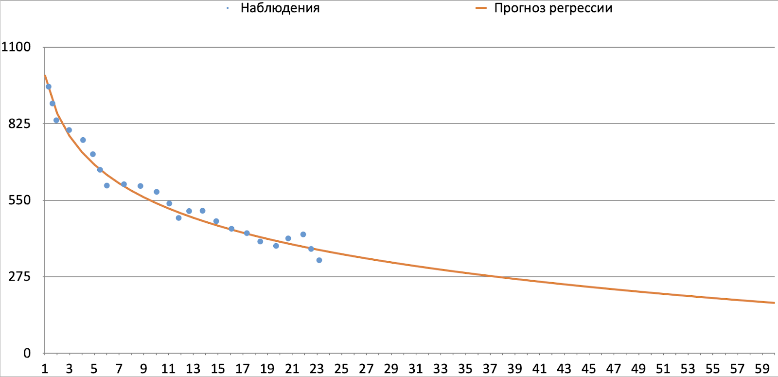
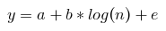
For each segment, we build a model that will describe the dependence of the CLTV component on the month of prediction by the equation
(you can do this in a loop, build a pairwise regression for each segment, or you can add a variable responsible for the segment to the equation and multiply it by x). To calculate the coefficients, we use the last 6 months of the forecast – 6 generations (where generation = a group of subscribers for whom a 24-month forecast is available for the month in question). Thus, the initial table is a list of subscribers for the last 6 months, their forecasts for each of the 6 months for 2 years in advance and a number of subscriber characteristics that allow us to determine which segment the subscriber belongs to.
We will build a pairwise regression for each segment in the cycle.
So, in each segment for each cohort we have a series of forecasts for 1,2,3,..12,…24 months ahead, we extrapolate it using the least squares method (we used statsmodels). We select the specification (formula of how y depends on x, logarithmically, linearly, exponentially…) of the equation based on the type of a number of predictors and a number of facts. To select the most suitable specification Ramsey test and other specification tests can be used.
The code below helps create a list of renewal coefficients for the selected segment of the segm segment, builds a summary and graph of the model for this segment, and you can conveniently view the main statistics of the model.
import numpy as np
import math
import pandas as pd
import statsmodels.api as sm
import statsmodels.formula.api as smf

# df - таблица с рядами суммарных прогнозов по сегментам
SEGM = '...' # выбранный сегмент для расчета
df_segm = df[df['segment'] == SEGM]

form_reg = '(service_margin) ~ 1 + np.log(period_key)'
model = smf.ols(formula=form_reg, data=df_segm)
result = model.fit()
# вынимаем a и b из y = a + b(ln(x))
a = result.params[0]
b = result.params[1]
# смотрим саммари
print(result.summary())

N_PRED_HORIZON = 24
y_fact = list(df_segm['service_margin'])
y_pred = []
for period in range(1,25):
    y_pred+=[a+b*np.log(period)]
for period in range(25,61):
    y_fact+=[a+b*np.log(period)]
    y_pred+=[a+b*np.log(period)]

segment_coeffs = y_pred[N_PRED_HORIZON:]/y_pred[N_PRED_HORIZON-1]

# строим прогноз и факт на 1 графике
print(segm)
plt.plot(y_fact, label="y_fact")
plt.plot(y_pred, label="y_pred")
plt.legend(loc="upper right")
plt.show()
At this stage, the coefficients of determination are controlled (

) and the adequacy of the coefficients of the constructed models. Next, we substitute for each segment and period from 25 to 60, we get the predicted

and divide it by

we get the coefficient for converting the forecast for the 24th month into a forecast for the selected period as in the code above.
Example: in the XXX segment, after applying the least squares method, we received the equation
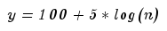
substitute into the equation

we get

divide by the forecast for the 24th period

and we get the coefficient

Instead of building a model for each segment, you can add to the equation a variable responsible for each segment and multiply it by the period. With 240 segments the equation would look something like this

where s1, s2,… are the active variables of the segments, take values 0 and 1. For each segment, only one variable s will be equal to 1, the rest will be zero, thus the problem will be reduced to the same paired regression as we built in the previous version .
4. Problems and approaches to their solution
Important variables are not taken into account. (endogeneity) This problem can arise if our CLTV component is highly dependent on some parameter. In our case, this parameter is the number of days in a month, which determines the amount of the monthly payment in tariffs with daily payment. This gives us a problem: the random error is no longer random, but depends on the number of days in the forecast month, so the coefficient estimates are not valid. In this case, we can divide our target variable by the number of days in the month and build models for the daily average component.
The time series of speeds does not repeat the features of a number of facts. This problem can arise if the model performs well on average, but overpredicts in some segments and underestimates in others. For example, in the graph below, a number of forecasts are decreasing, while a number of facts are increasing. In such a case, we extended with a moving average.
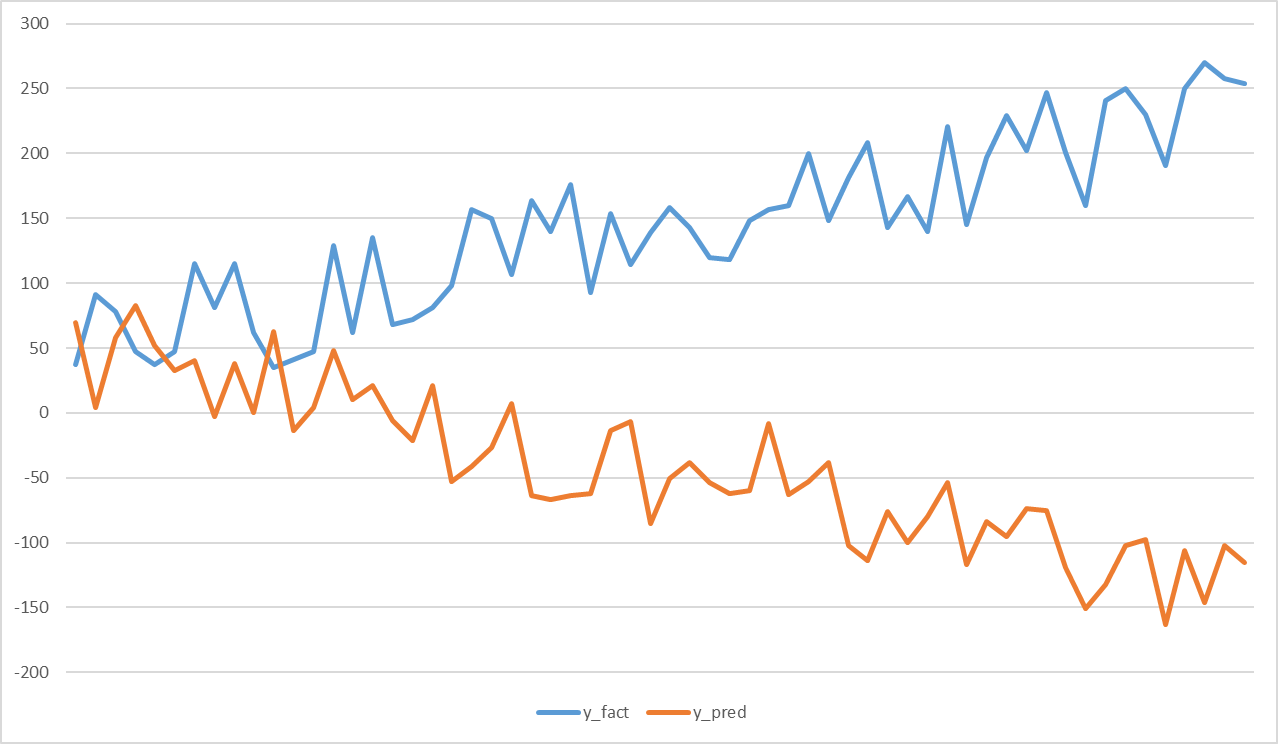
Hidden text
x | y_fact | y_pred |
1 | 37 | 70 |
2 | 91 | 4 |
3 | 78 | 58 |
4 | 47 | 83 |
5 | 37 | 52 |
6 | 47 | 33 |
7 | 115 | 40 |
8 | 81 | -3 |
9 | 115 | 38 |
10 | 62 | 0 |
eleven | 35 | 63 |
12 | 41 | -14 |
13 | 47 | 4 |
14 | 129 | 48 |
15 | 62 | 10 |
16 | 135 | 21 |
17 | 68 | -6 |
18 | 72 | -21 |
19 | 81 | 21 |
20 | 98 | -53 |
21 | 157 | -41 |
22 | 150 | -27 |
23 | 107 | 7 |
24 | 164 | -64 |
25 | 140 | -67 |
26 | 176 | -64 |
27 | 93 | -62 |
28 | 154 | -14 |
29 | 114 | -7 |
thirty | 139 | -85 |
31 | 158 | -51 |
32 | 143 | -38 |
33 | 120 | -54 |
34 | 118 | -62 |
35 | 148 | -60 |
36 | 157 | -8 |
37 | 160 | -63 |
38 | 200 | -53 |
39 | 148 | -38 |
40 | 181 | -102 |
41 | 208 | -114 |
42 | 143 | -76 |
43 | 167 | -100 |
44 | 140 | -80 |
45 | 221 | -54 |
46 | 145 | -117 |
47 | 197 | -84 |
48 | 229 | -95 |
49 | 202 | -74 |
50 | 247 | -75 |
51 | 201 | -119 |
52 | 160 | -151 |
53 | 241 | -132 |
54 | 250 | -102 |
55 | 230 | -98 |
56 | 191 | -163 |
57 | 250 | -106 |
58 | 270 | -146 |
59 | 258 | -102 |
60 | 254 | -115 |
3. The first 1-3 months of the forecast “jump” or have a different character of the curve. (convex upward). This problem occurs for fresh and inactive subscribers, because the models work worse for them. In this case, you can extrapolate the series starting from the 4-5th month of the forecast, or you can calculate a moving average with a window of 3 months and build statistical models on it.
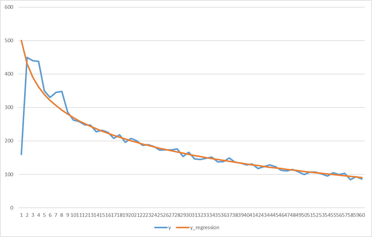
Hidden text
y | y_regression | |
1 | 160 | 500 |
2 | 450 | 430.6853 |
3 | 440 | 390.1388 |
4 | 438 | 361.3706 |
5 | 350 | 339.0562 |
6 | 330 | 320.8241 |
7 | 345 | 305.409 |
8 | 348 | 292.0558 |
9 | 287.2775 | 280.2775 |
10 | 262.7415 | 269.7415 |
eleven | 258.2105 | 260.2105 |
12 | 248.5093 | 251.5093 |
13 | 247.5051 | 243.5051 |
14 | 227.0943 | 236.0943 |
15 | 232.195 | 229.195 |
16 | 225.7411 | 222.7411 |
17 | 207.6787 | 216.6787 |
18 | 217.9628 | 210.9628 |
19 | 195.5561 | 205.5561 |
20 | 207.4268 | 200.4268 |
21 | 200.5478 | 195.5478 |
22 | 186.8958 | 190.8958 |
23 | 188.4506 | 186.4506 |
24 | 183.1946 | 182.1946 |
25 | 172.1124 | 178.1124 |
26 | 173.1903 | 174.1903 |
27 | 173.4163 | 170.4163 |
28 | 175.7795 | 166.7795 |
29 | 153.2704 | 163.2704 |
thirty | 165.8803 | 159.8803 |
31 | 146.6013 | 156.6013 |
32 | 144.4264 | 153.4264 |
33 | 148.3492 | 150.3492 |
34 | 151.3639 | 147.3639 |
35 | 137.4652 | 144.4652 |
36 | 138.6481 | 141.6481 |
37 | 148.9082 | 138.9082 |
38 | 136.2414 | 136.2414 |
39 | 133.6438 | 133.6438 |
40 | 128.1121 | 131.1121 |
41 | 130.6428 | 128.6428 |
42 | 117.233 | 126.233 |
43 | 122.88 | 123.88 |
44 | 128,581 | 121,581 |
45 | 123.3338 | 119.3338 |
46 | 112.1359 | 117.1359 |
47 | 109.9852 | 114.9852 |
48 | 114.8799 | 112.8799 |
49 | 107,818 | 110,818 |
50 | 99.7977 | 108.7977 |
51 | 106.8174 | 106.8174 |
52 | 106.8756 | 104.8756 |
53 | 100.9708 | 102.9708 |
54 | 95.1016 | 101.1016 |
55 | 105.2667 | 99.26668 |
56 | 99.46483 | 97.46483 |
57 | 102.6949 | 95.69487 |
58 | 83.9557 | 93.9557 |
59 | 93.24626 | 92.24626 |
60 | 85.56554 | 90.56554 |
So far we have discussed which extrapolation approaches can be used to extend forecasts out to a 5-year horizon. The guys from the Beeline CLTV team will talk about what to do next with these indicators, as well as about the features of forecasting CLTV components very soon in the following articles.