Bayesian Ranking by Dr. Kübler

Imagine that in

some

The game players compete one on one. A natural question arises: “How to rank them?”. For an answer, we invite you under the cut – to the start of our

flagship course in Data Science

.

Let’s see how to build a ranking model for a set of players (recommendations, search results

etc.

). We will do this using a Bayesian model, where the ranking is performed even without the characteristics of the players themselves, although their accounting can be added.

Theoretically, the task should not become too difficult: let the players play several times and look at the ratio of wins. But, unfortunately, this natural approach is not ideal. That’s why:

• it is impossible to determine what exactly a ratio of wins close to 100% means: either the player is exceptional, or only weak opponents lost to him;
• if a player has played only a few games, then there is a high uncertainty in assessing his strength. With a “raw” ratio of wins, this problem does not exist.

Tasks that are formulated as one-on-one games are often encountered in rankings. This applies to:

• players in real competition: tennis, racing, card games, pokemon fights etc.
• search results: the more relevant they are to the user’s query, the better;
• recommendations: the more relevant they are to what the user wants to buy, the better, etc.

Let’s use PyMC to create a simple Bayesian model that solves this ranking problem. Model details

see

in my introduction to the Bayesian world with PyMC, a precursor to PyMC with much the same syntax.

Model Bradley – Terry

Let’s give

this model

Bayesian sound. Scary, but really very simple.

What is this model?

This whole model boils down to two assumptions:

1. Each player (human, pokemon) has a game power, search results and recommendations have relevance, and so on.
2. If players 1 and 2 compete, whose strength s₁ and s₂ respectively, player 1 wins with the following probability:

σ – our good old sigmoid

Moreover, no signs (characteristics) of players such as height or weight of a person are used here. So, this model is applicable to different tasks.

If you include the characteristics of the players in it, you can get something like Microsoft RankNet. To out signs x explicitly construct the numerical values ​​of the strength of the players s = f(x)the authors of RankNet use a neural network, and in the Bayesian approach, the forces s directly work as parameters.

To build a frequency version of the Bradley-Terry model using a deep learning framework, you can use an embedding layer. Let’s check the performance of such a model building. So, each player has a power. According to it, the players are ordered.

Suppose the first player has much more strength than the second, that is, s₁ — s₂ is a big number. Means, σ(s₁ — s₂) close to unity. Thus, with a huge probability, the first player will win. This is exactly what we need here. In the opposite situation – similarly. If the players have the same strength, the probability of winning for each of them is equal to σ(0) = 50%. Perfect.

Create a dataset

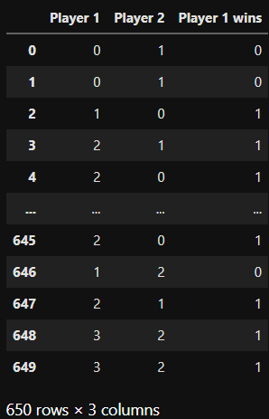
Before building the model, let’s create an artificial dataset about game results:

And now we have an advantage: we know the features to look for in the model.

Here is the artificial data generation code:

import pandas as pd
import numpy as np
np.random.seed(0)
def determine_winner(player_1, player_2):
    if player_1 == 0 and player_2 == 1:
        return np.random.binomial(n=1, p=0.05)
    if player_1 == 0 and player_2 == 2:
        return np.random.binomial(n=1, p=0.05)
    if player_1 == 1 and player_2 == 0:
        return np.random.binomial(n=1, p=0.9)
    if player_1 == 1 and player_2 == 2:
        return np.random.binomial(n=1, p=0.1)
    if player_1 == 2 and player_2 == 0:
        return np.random.binomial(n=1, p=0.9)
    if player_1 == 2 and player_2 == 1:
        return np.random.binomial(n=1, p=0.85)
games = pd.DataFrame({
    "Player 1": np.random.randint(0, 3, size=1000),
    "Player 2": np.random.randint(0, 3, size=1000)
}).query("`Player 1` != `Player 2`")
games["Player 1 wins"] = games.apply(
    lambda row: determine_winner(row["Player 1"], row["Player 2"]),
    axis=1
)

The set consists of data about three players who compete against each other randomly. This is exactly what happens in the function

determine_winner

: two player indices are accepted

(0, 1, 2)

and the output is shown if wins

player_1

. Example: in game

(0, 1)

player 0 wins with probability

p=0.05

player 1.

Take a close look at the probabilities in the code: player 2 should be the best, 1 the average, and 0 the weakest.

For variety, let’s introduce a fourth player who played only two games:

new_games = pd.DataFrame({
    "Player 1": [3, 3],
    "Player 2": [2, 2],
    "Player 1 wins": [1, 1]
})
games = pd.concat(
    [games, new_games],
    ignore_index=True
)

Player 3 played twice against number 2 and even won twice. This means that number 3 must also have a high strength value. But it is impossible to say whether he is really better than number 2 or if it was an accident.

Model building with RUMS

Now we can build the model. Note that the strengths of the players are denoted by Gaussian priors. In addition, the model displays posterior values ​​for five players, although there is no data for the last player number 4. Let’s see how it goes.

More importantly, I don’t explicitly use the sigmoid. If we pass the difference in the strength of the game among the players through the parameter logit_pbut not pthe role of the sigmoid will be played by the object pm. Bernoulli.

import pymc as pm
with pm.Model() as model:
    strength = pm.Normal("strength", 0, 1, shape=5)
    diff = strength[games["Player 1"]] - strength[games["Player 2"]]
    
    obs = pm.Bernoulli(
        "wins",
        logit_p=diff,
        observed=games["Player 1 wins"]
    )
    
    trace = pm.sample()

Let’s check how the posterior values ​​are distributed. Above – posterior distributions in the form of density plots, below – a forest diagram [forest plot]on which it is easy to compare the posterior values ​​of the force:

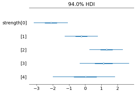
Look, player number 0 is indeed the weakest, followed by number 1. Numbers 2 and 3 are the best, as expected. The mean of the posterior distribution for number 3 is slightly lower than for number 2. But the interval of high density is much larger. That is, the uncertainty about the strength of number 3 is greater compared to number 2. The posterior value of the strength of number 4 is the same as the a priori. It is normally distributed with a mean of 0 and a standard deviation of 1. Nothing new can be taught to the model here. Here are some more numbers:

It seems that in this case a good convergence of MCMC was also observed: all values r_hat are equal to 1.

Also, some players have a negative strength value, but that’s okay, because we’re only using the difference in strength between the two players anyway. If this is for you some reason you don’t like it, replace the prior values ​​of the force with a semi-normal distribution HalfNormal or simply add a constant to the posterior values, such as 5. Then all the averages and high density intervals will be in the positive range.

Conclusion

The model began with a priori ideas about the levels of the game’s strength, which were then changed with the help of data. The more games played, the less uncertainty about the strength of the player. In the extreme case, when the player has not played a single game, the posterior distribution of his strength is equal to the a priori one, which is logical.

I hope you learned something new, interesting and useful today. Thank you for your attention!

And we will help you understand programming so that you can boost your career or become a sought-after IT professional:

To see all courses, click on the banner: