Solving the problem of determining RUL transformers using machine learning in python

In the same article, a common approach to solving the problem of determining RUL based on regression modelssince we have diagnostic data (time series, signals) and markup in the form of equipment duration to failure values.

2. Download data

Loading Libraries

import numpy as np
import pandas as pd
from matplotlib import pyplot as plt

PATH = '/kaggle/input/transformer-time/'

Loading the markup of the training sample

We have a markup file (essentially a dictionary), which presents data on the residual time of the transformer to failure: each file with gas concentrations corresponds to 1 number – the remaining time to failure at the end of the file.

y_data = pd.read_csv(PATH + 'train.csv', index_col="id")
y_data.head()

Where:

• id – the name of the file that is in PATH with time-varying transformer parameters.

• predicted – Remaining time until equipment failure

Loading the training sample (transformer parameters)

Let’s load all files with time-varying transformer parameters (gas concentrations) into a dictionary, where the key is the file name. In this case, we will only load those files for which there is a markup (the remaining time before failure).

X_data = {}
for row in y_data.iterrows():
    file_name = row[0]
    path = PATH + f'data_train/data_train/{file_name}'
    X_data[file_name] = pd.read_csv(path)

• Size of each file: (420, 4)

• Total number of markup files: 2100

The first 2 lines of each file look something like this:

X_data[file_name].head(2)

A training sample with markup and X_test without correct answers (markup) is available on Kaggle. For the purpose of demonstrating the possibility and quality of solving the problem, we will use only the Training set. We will divide it into training and validation (deferred) samples for training and testing the resulting models.

3. Simulation

Loading Libraries

from sklearn.model_selection import train_test_split
from sklearn.linear_model import LinearRegression, LogisticRegression
from sklearn.preprocessing import StandardScaler
from sklearn.metrics import mean_absolute_error, f1_score
from catboost import CatBoostRegressor
from tsfresh.feature_extraction import extract_features, MinimalFCParameters

Baseline Mean RUL

As the simplest baseline without machine learning, we take the average value on the training set and use it to predict the residual resource. To do this, implement the following pipeline:

1. Dividing the sample into training and validation

2. Calculation of the average value of the residual resource on the training sample and building a forecast by the average

3. Evaluation of the quality of the model on the validation set

At the beginning, we will clearly demonstrate all the steps (further the code will be under the cut):

1. First, we divide the sample into training and test

y_train, y_val = train_test_split(y_data, test_size=0.25, random_state=1)
print(f'Train set shape: {y_train.shape}')
print(f'Test set shape: {y_val.shape}')

Train set shape: (1575, 1)

Test set shape: (525, 1)

2. Next, we calculate the average and build a forecast

y_train_pred = [y_train.mean().values[0]] * len(y_train)
y_val_pred = [y_train.mean().values[0]] * len(y_val)

3. Let’s calculate the metrics

mae_train = round(mean_absolute_error(y_train, y_train_pred), 2)
mae_val = round(mean_absolute_error(y_val, y_val_pred), 2)
print(f'MAE on train set = {mae_train}')
print(f'MAE on test set = {mae_val}')

MAE on train set = 219.97

MAE on test set = 218.38

We have received the first metrics from which we can build. If machine learning models cannot significantly improve the metrics, then their use does not make sense.

Regression model approach

Let’s try something more complex and with machine learning. We implement the following pipeline for different aggregation options and models:

1. Data aggregation (simple aggregation/aggregation using TSFresh)

2. Dividing the sample into training and validation

3. Data normalization (if necessary)

4. Model training (linear regression/gradient boosting)

5. Model inference

6. Evaluation of the quality of the model on the validation set

Approach 1: Simple aggregation (average) + Linear regression

Simple aggregation means averaging parameters across columns within each file (4 mean values ​​on 4 features, respectively). For each one-dimensional time series, 1 number is obtained – the average over the series. That is, for each file we get 4 features (4 averages from 4 time series).

y = y_data.copy()
X = pd.concat([X_data[file].mean() for file in y_data.index], axis=1).T
X.index = y.index
X = X.add_suffix('_mean')

X_train, X_val, y_train, y_val = train_test_split(X, y, test_size=0.25, random_state=1)

StSc = StandardScaler()
X_train_sc = StSc.fit_transform(X_train)
X_val_sc = StSc.transform(X_val)

lr = LinearRegression()
lr.fit(X_train_sc, y_train)

y_train_pred = lr.predict(X_train_sc)
y_val_pred = lr.predict(X_val_sc)

mae_train = round(mean_absolute_error(y_train, y_train_pred), 2)
mae_val = round(mean_absolute_error(y_val, y_val_pred), 2)
print(f'MAE on train set = {mae_train}')
print(f'MAE on test set = {mae_val}')

MAE on train set = 177.7

MAE on test set = 175.12

Approach 2: Simple aggregation (medium) + Gradient boosting (CatBoost)

y = y_data.copy()
X = pd.concat([X_data[file].mean() for file in y_data.index], axis=1).T
X.index = y.index
X = X.add_suffix('_mean')

X_train, X_val, y_train, y_val = train_test_split(X, y, test_size=0.25, random_state=1)

cbr = CatBoostRegressor(random_state=1, verbose=0)
cbr.fit(X_train, y_train)

y_train_pred = cbr.predict(X_train)
y_val_pred = cbr.predict(X_val)

mae_train = round(mean_absolute_error(y_train, y_train_pred), 2)
mae_val = round(mean_absolute_error(y_val, y_val_pred), 2)
print(f'MAE on train set = {mae_train}')
print(f'MAE on test set = {mae_val}')

MAE on train set = 100.6

MAE on test set = 161.67

Approach 3: Data Aggregation with TSFresh + Linear Regression

Library for aggregation and feature extraction from time series TSFresh allows you to select much more complex features compared to a simple average. We will use the minimum 10 features for demonstration: sum, median, mean, length, std, variance, RMS, max, abs_max, min.

X = pd.concat([X_data[file].assign(id=file) for file in y_data.index], axis=0, ignore_index=True)
y = y_data.copy()

settings = MinimalFCParameters()
X = extract_features(X, 
                     column_id="id", 
                     default_fc_parameters=settings).loc[y.index]

X_train, X_val, y_train, y_val = train_test_split(X, y, test_size=0.25, random_state=1)

StSc = StandardScaler()
X_train_sc = StSc.fit_transform(X_train)
X_val_sc = StSc.transform(X_val)

lr = LinearRegression()
lr.fit(X_train_sc, y_train)

y_train_pred = lr.predict(X_train_sc)
y_val_pred = lr.predict(X_val_sc)

mae_train = round(mean_absolute_error(y_train, y_train_pred), 2)
mae_val = round(mean_absolute_error(y_val, y_val_pred), 2)
print(f'MAE on train set = {mae_train}')
print(f'MAE on test set = {mae_val}')

MAE on train set = 140.82

MAE on test set = 148.21

Approach 4: Data Aggregation with TSFresh + Gradient Boosting (CatBoost)

X = pd.concat([X_data[file].assign(id=file) for file in y_data.index], axis=0, ignore_index=True)
y = y_data.copy()

settings = MinimalFCParameters()
X = extract_features(X, 
                     column_id="id", 
                     default_fc_parameters=settings).loc[y.index]

X_train, X_val, y_train, y_val = train_test_split(X, y, test_size=0.25, random_state=1)

cbr = CatBoostRegressor(random_state=1, verbose=0)
cbr.fit(X_train, y_train)

y_train_pred = cbr.predict(X_train)
y_val_pred = cbr.predict(X_val)

mae_train = round(mean_absolute_error(y_train, y_train_pred), 2)
mae_val = round(mean_absolute_error(y_val, y_val_pred), 2)
print(f'MAE on train set = {mae_train}')
print(f'MAE on test set = {mae_val}')

MAE on train set = 37.2

MAE on test set = 91.37

The model error decreases as the algorithm becomes more complex, but still not strong enough. Despite the good metrics of the last approach, the model showed significant overfitting, so its results should be treated with caution.

Let’s look at the distribution of the model’s predictions and correct answers to assess where the model is wrong in order to understand how the algorithm for solving the problem can be changed.

plt.figure(figsize=(6, 3))
plt.hist(y_val_pred, bins=30, alpha=0.6, label="Predicted values on the test set")
plt.hist(y_val, bins=30, alpha=0.6, label="True values of the test set")
plt.legend()
plt.show()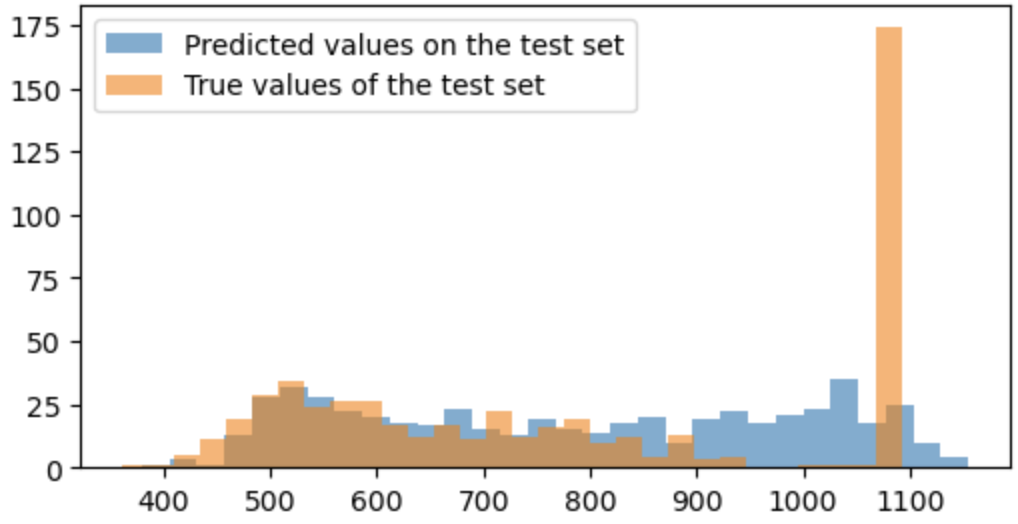

You can see that the model is quite wrong on cases when the value is 1093 (the tall orange bar on the right side of the graph). This is the limit value, above which the residual resource is set to a constant value of 1093, that is, the residual resource is quite large, and it is not necessary to determine the exact value from the point of view of diagnostic purposes.

Ensemble approach (classification+regression)

To reduce the error and solve the problem of models with misunderstanding and the inability to fairly accurately predict the value of 1093. To do this, before predicting the value of the residual life by the regression model, we put a classification model that will say whether the state of the transformer belongs to one of the options: “RUL=1093” or “RUL<1093". No data “RUL>1093”, since the data is already pre-processed before us. We implement the following pipeline for different aggregation options and models:

1. Data aggregation with TSFresh

2. Dividing the sample into training and validation

3. Data normalization (if necessary)

4. Training a binary classification model (0 – “RUL<1093"; 1 – “RUL=1093”)

5. Training a regression model (linear regression/gradient boosting) on ​​data “RUL<1093"

6. Binary Classification Model Inference

7. Regression model inference on data where the classification model predicted 0

8. Evaluation of the quality of the model on the validation set

Approach 1: TSFresh + Logistic Regression + Linear Regression

y = (y_data == 1093).astype(int)
X = pd.concat([X_data[file].assign(id=file) for file in y_data.index], axis=0, ignore_index=True)

settings = MinimalFCParameters()
X = extract_features(X, 
                     column_id="id", 
                     default_fc_parameters=settings).loc[y.index]

X_train, X_val, y_train, y_val = train_test_split(X, y, test_size=0.25, random_state=1)

StSc = StandardScaler()
X_train_sc = StSc.fit_transform(X_train)
X_val_sc = StSc.transform(X_val)

LogReg = LogisticRegression()
LogReg.fit(X_train_sc, y_train)

y_train_pred_outliers = pd.DataFrame(LogReg.predict(X_train_sc), 
                                     index=y_train.index, 
                                     columns=y_train.columns)
y_val_pred_outliers = pd.DataFrame(LogReg.predict(X_val_sc), 
                                   index=y_val.index, 
                                   columns=y_val.columns)

f1_train = round(f1_score(y_train, y_train_pred_outliers), 2)
f1_val = round(f1_score(y_val, y_val_pred_outliers), 2)
print(f'F1 on train set = {f1_train}')
print(f'F1 on test set = {f1_val}')

F1 on train set = 0.67

F1 on test set = 0.64

Classification metrics can be greatly improved!

y = y_data.copy()

X_train, X_val, y_train, y_val = train_test_split(X, y, test_size=0.25, random_state=1)

y_train_wo_outliers = y_train[y_train != 1093].dropna()
X_train_wo_outliers = X_train.loc[y_train_wo_outliers.index]

StSc = StandardScaler()
X_train_wo_outliers_sc = StSc.fit_transform(X_train_wo_outliers)
X_train_sc = StSc.transform(X_train)
X_val_sc = StSc.transform(X_val)

lr = LinearRegression()
lr.fit(X_train_wo_outliers_sc, y_train_wo_outliers)

y_train_pred = pd.DataFrame(lr.predict(X_train_sc), 
                            index=y_train.index, 
                            columns=y_train.columns)
y_val_pred = pd.DataFrame(lr.predict(X_val_sc), 
                          index=y_val.index, 
                          columns=y_val.columns)

ind = y_train_pred_outliers[y_train_pred_outliers['predicted']==1].index
y_train_pred.loc[ind] = 1093

ind = y_val_pred_outliers[y_val_pred_outliers['predicted']==1].index
y_val_pred.loc[ind] = 1093

mae_train = round(mean_absolute_error(y_train, y_train_pred), 2)
mae_val = round(mean_absolute_error(y_val, y_val_pred), 2)
print(f'MAE on train set = {mae_train}')
print(f'MAE on test set = {mae_val}')

MAE on train set = 133.12

MAE on test set = 137.01

Of course, we have improved the result compared to the usual linear regression model, but this is still not enough.

Approach 2: TSFresh + Logistic Regression + Gradient Boosting

Stage 1 – the classification remains the same, the code does not change, so we present the code only for stage 2:

y = y_data.copy()

X_train, X_val, y_train, y_val = train_test_split(X, y, test_size=0.25, random_state=1)

y_train_wo_outliers = y_train[y_train != 1093].dropna()
X_train_wo_outliers = X_train.loc[y_train_wo_outliers.index]

StSc = StandardScaler()
X_train_wo_outliers_sc = StSc.fit_transform(X_train_wo_outliers)
X_train_sc = StSc.transform(X_train)
X_val_sc = StSc.transform(X_val)

cbr = CatBoostRegressor(random_state=1, verbose=0)
cbr.fit(X_train_wo_outliers_sc, y_train_wo_outliers)

y_train_pred = pd.DataFrame(cbr.predict(X_train_sc), 
                            index=y_train.index, 
                            columns=y_train.columns)
y_val_pred = pd.DataFrame(cbr.predict(X_val_sc), 
                          index=y_val.index, 
                          columns=y_val.columns)

ind = y_train_pred_outliers[y_train_pred_outliers['predicted']==1].index
y_train_pred.loc[ind] = 1093

ind = y_val_pred_outliers[y_val_pred_outliers['predicted']==1].index
y_val_pred.loc[ind] = 1093

mae_train = round(mean_absolute_error(y_train, y_train_pred), 2)
mae_val = round(mean_absolute_error(y_val, y_val_pred), 2)
print(f'MAE on train set = {mae_train}')
print(f'MAE on test set = {mae_val}')

MAE on train set = 77.11

MAE on test set = 106.49

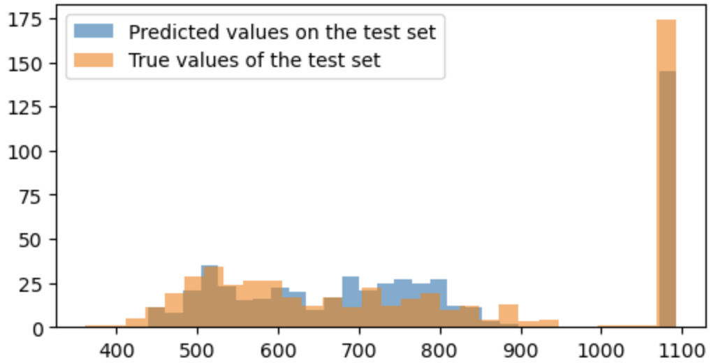
Despite the deterioration in the quality of the model compared to a similar approach without the classification stage, it can be stated that the results of the model improved due to the reduction in overfitting.

Conclusion

We have considered only one common approach to solving the problem. We made several hypotheses about the methods and data, and tested them. The overall results are shown in the picture below.

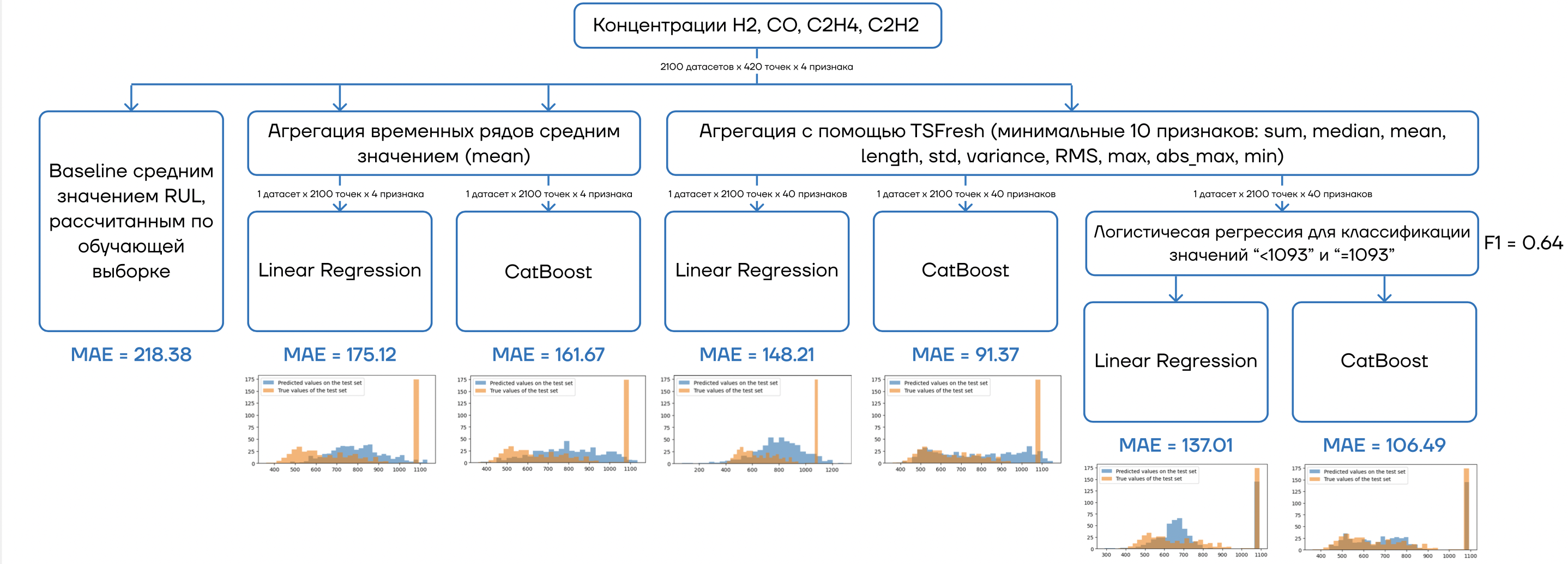
By the way, the result can be improved by 2-3 times (error reduction) compared to the one obtained in the article, so you can try! In addition, there are still quite a few hypotheses to test, for example:

1. Extension of the feature set by means TSFresh (up to several thousand signs. by subsequent selection)

2. Training regression models after classification not on data “RUL<1093"but for all

3. Using the results of a classification model as a feature for the input of regression models

4. Using a more complex classification model to improve the quality of case separation “RUL=1093” And “RUL<1093"

5. (Fundamentally different approach to setting and solving the problem) STO 34.01-23-003-2019)

6. and many others

I created telegram channel DataKatser, where I appear much more often and share my thoughts and interesting cases on data science, machine learning and artificial intelligence. I will be glad to your subscription!