Optimizing Jupyter Notebook Performance with Parallel Computing (Joblib Library)

NTA professional community.

In this post, I will talk about the possibilities of using parallel computing in an interactive environment. jupyter notebook language Python.

Quick post navigation

Why do we need parallelism?

Parallelism plays an important role in Data Science tasks, as it can significantly speed up calculations and processing of large amounts of data. Here are some main reasons why multiprocessing is important for these tasks:

Computation accelerationA: Many tasks in DS such as training machine learning models, clustering, image processing, and big data analysis are computationally intensive. The use of parallel computing allows you to distribute work among several processor cores or even between several computers, which leads to a significant acceleration of task execution.
Big Data Processing: Parallel computing allows you to effectively parallelize data processing by dividing it into smaller parts and executing them simultaneously.
Hyperparameter optimization: due to the parallel execution of experiments with different values of hyperparameters, you can speed up the process of finding the optimal parameters of the model.
Streaming Data Processing: It may be necessary to process real-time streaming data. Multiprocessing allows you to efficiently process and analyze data streams, especially in the case of high loads and the need for real-time data processing.

Python already has an implementation of concurrency based on the base module — multiprocessing. Then why won’t it work in Jupyter notebook?

Why doesn’t multiprocessing work?

Jupyter Notebook is having issues when using multiprocessing module due to its interaction with the Jupyter interactive environment. These issues are because Jupyter Notebook runs the Python kernel in its own process, which is already executing cell code.

multiprocessing module Python uses process forking to achieve parallel execution. However, the Jupyter Notebook already has a running Python process, and when trying to use multiprocessing in a cell, an attempt is made to create a new child process within an already existing process, which causes a conflict.

It should also be noted that Jupyter Notebook itself is an interactive environment where you can execute code in cells in any order and at any time. However multiprocessing requires code to be executed in the main (main) module of the program, which makes it difficult to work with Jupyter Notebook.

Joblib vs. multiprocessing

Library joblib provides a simple interface for executing tasks in parallel on multiple processor cores, and it can be used in Jupyter Notebook to enable parallelism.

The main difference between multiprocessing And joblib is how they interact with the Python interpreter. Unlike multiprocessing, joblib uses background processes that run independently of the main Jupyter Notebook process. Thus, joblib avoids the problems associated with creating child processes within an already existing process.

Let’s move on to a practical demonstration of the code without the use of parallel computing.

Monkey sort without parallel computing

First you need to simulate a computational function with a long execution, of the most famous and simple options, this is monkey sort – a sorting algorithm that checks whether the array is sorted, if not, then randomly shuffle until it is sorted. Its average asymptotic will be O((n+1)!), on average, because there is a random factor and mixing can happen both faster and longer, but when applying the law of large numbers, the asymptotic tends to this value.

Import the required libraries:

from joblib import Parallel, delayed
import pandas as pd
import random
import numpy as np
import warnings
import random

warnings.filterwarnings('ignore')

Implementing the Fastest Sort Algorithm bogosort (monkey sort) in Python language:

def bogosort(arr):
    def correct(arr, comparator=lambda x: x):
        for i in range(1, len(arr)):
            if comparator(arr[i - 1]) - comparator(arr[i]) > 0:
                return False
        
        return True

    while not correct(arr):
        random.shuffle(arr)
    
    return arr

To test hypotheses, we will generate a two-dimensional array, which will contain 8 randomly located integer values and a total of 1000 such sets:

bigdata = np.array([[random.randint(0, 100) for _ in range(8)] for _ in range(1000)])
print(bigdata[:5]) # выводим первые 5 элементов

You can check the operation of the algorithm on this data set; to account for time, we use the built-in Python magic function%%time:

%%time
bg = bigdata.copy()
order_bg = list(map(bogosort, bg))

Let’s check the results:

print(order_bg[:5]) # выводим первые 5 элементов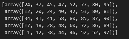

Everything was successfully sorted in 4 minutes 32 seconds.

And if you apply multiprocessing?

Now let’s solve the same problem by applying multiprocessing.

It should be noted that a different approach to the implementation of functions is needed here, we will single out 2 approaches within the framework of this task:

First approach consists in the decomposition of the problem and the parallel execution of computational iterations. However, in a particular case, we have only one subtask – random mixing. Dividing this task into parallel parts does not make sense because the processor will spend time coordinating and synchronizing parallel processes, which can increase overhead and slow down execution.
Instead, I suggest second approach – use of dividing data into partitions and performing calculations for each of them. This approach is similar to the methods used in Apache Spark.

Let’s move on to writing the code for the second option, in this case the function will be kept original, and we do not need to isolate the process, and then synchronize it with the general data collection queue, this allows us to do joblib And lambda python functions:

N_CORES = 12 # количество задействованных ядер процессора

list_array = np.array_split(bigdata, N_CORES)
data = Parallel(n_jobs=N_CORES, verbose=10)(delayed(lambda array: list(map(bogosort, array)))(array) for array in list_array)

joblib provides a class parallel, which allows you to distribute the execution of loop iterations or function calls to multiple processor cores. It can use various concurrency techniques, including the use of processes or threads. In function argument delayed I designate a function, of course, without a call. Next should mention the argument for filing in pipeline functions and the object from which we will take it. All this is done in the list comprehended format.

Apart from lambdafor readability, we can declare a function multi_bogosort:

def multi_bogosort(ndarray):
    return list(map(bogosort, ndarray))

And then the final version with it will look like this:

N_CORES = 12

list_array = np.array_split(bigdata, N_CORES)
data = Parallel(n_jobs=N_CORES, verbose=10)(delayed(multi_bogosort)(array) for array in list_array)

note that joblib automatically handles data splitting and result collection so you don’t have to worry about explicit process or thread management.

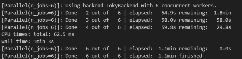
Let’s look at the execution time:

We see a significant acceleration, but in reality not everything is so “perfect”, the data format has changed a little and we need to merge them again after separation, for example, using the following algorithm:

from functools import reduce

merge_data = reduce(lambda x, y: x.extend(y) or x, data)

And let’s check the data as usual:

merge_data[:5]

Due to the inclusion of additional pre-processing and post-processing of the results, as well as the coordination and synchronization of processors, we spend some time, and therefore the result will not have a pure t / N_cores dependence.

The final acceleration of the process from 4 minutes 32 seconds (272 seconds) versus 44.9 seconds, and this is a 6-fold increase in productivity.

Let’s also do a test for 6 processors for comparison:

%%time

N_CORES = 6

list_array = np.array_split(bigdata, N_CORES)
data = Parallel(n_jobs=N_CORES, verbose=10)(delayed(multi_bogosort)(array) for array in list_array)
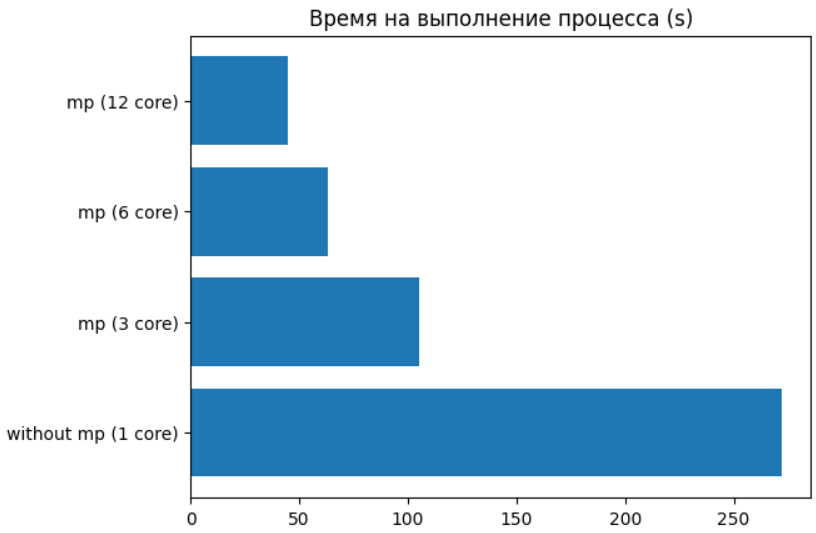
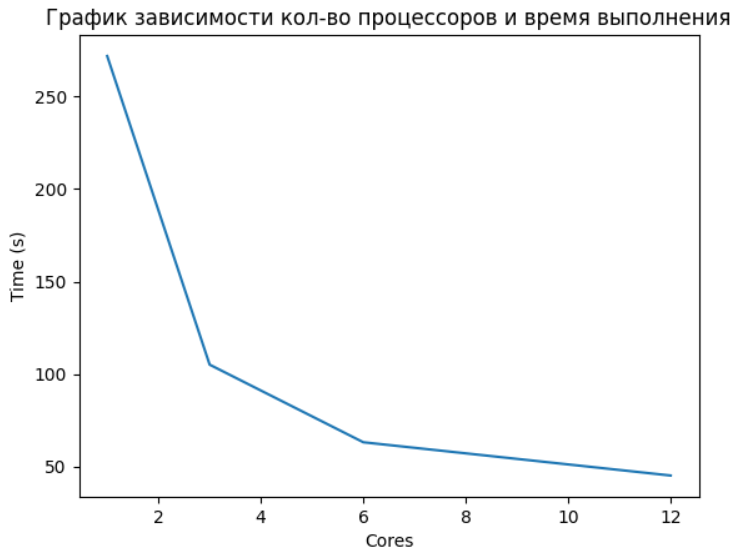
merge_data = reduce(lambda x, y: x.extend(y) or x, data)

Below you can see the dependence of execution time on the number of processor cores used for a parallel function. (It is important to note that the item with 12 cores should be understood as 6 physical + 6 logical, and therefore did not see a significant increase, because 6 logical cores are threads, and the GIL is already affecting here).

The use of parallel computing can bring significant benefits in the tasks of data analysis and machine learning. This is especially important when working with really large amounts of data. Often in the work of specialists in the field of Data Science, the most used tools are interactive environments. Jupyter, this is due to the ease of experiments and testing in it. And without the ability to use parallelism, the functionality is limited, and in this case, we are rescued by the very joblib.

I would like to add one more example on a real problem in RL, when we need to find the optimal number of clusters using the so-called elbow method. Briefly: the algorithm works as follows, calculates the KMeans model iteratively for a specific search area. After that, it calculates a certain metric, in this case I will use a silhouette. And as a result, we determine the optimal metric when an increase in clusters does not give a significant increase, interpreting these statements into a graph, we get something like an elbow bend, when the errors become relatively smooth.

Expand Code

from sklearn.cluster import KMeans
from sklearn.datasets import make_blobs
from sklearn.metrics import silhouette_score
from sklearn import preprocessing
from sklearn.decomposition import PCA
from sklearn.pipeline import Pipeline
from sklearn.base import BaseEstimator, TransformerMixin
from sklearn.model_selection import GridSearchCV

class KMeansWithSilhouette(BaseEstimator, TransformerMixin):
    def __init__(self, n_clusters):
        self.n_clusters = n_clusters

    def fit(self, X, y=None):
        self.kmeans = KMeans(n_clusters=self.n_clusters)
        self.kmeans.fit(X)
        return self

    def transform(self, X):
        return self.kmeans.transform(X)

    def score(self, X, y=None):
        labels = self.kmeans.predict(X)
        return silhouette_score(X, labels)

def calculate_silhouette_scores(X, cluster_range):
    pipeline = Pipeline([
        ('scaling', preprocessing.StandardScaler()),
        ('pca', PCA(n_components=2)),
        ('kmeans', KMeansWithSilhouette(n_clusters=cluster_range))
    ])

    grid_search = GridSearchCV(pipeline, param_grid={}, cv=5, n_jobs=1)
    grid_search.fit(X)
    return grid_search.best_score_

Let’s implement the calculation function, without parallel execution, also for the test we will take randomly generated data with 7 centroids.

def calculate_elbow(X, cluster_range):
    silhouette_scores = []
    for n in cluster_range:
        score = calculate_silhouette_scores(X, n)
        silhouette_scores.append(score)

    deltas = np.diff(silhouette_scores)
    elbow_index = np.argmax(deltas) + 1

    return cluster_range[elbow_index]

X, _ = make_blobs(n_samples=10000, n_features=100, centers=7, random_state=42)
cluster_range = range(2, 15)

start_time = time.time()
elbow_value = calculate_elbow(X, cluster_range)
elapsed_time = time.time() - start_time

print("The optimal number of clusters is:", elbow_value)
print("Execution time:", elapsed_time, "seconds")

In 15.5 seconds, I calculated 15 clusters and chose the optimal number = 3. Now we will do this using joblib.

def calculate_elbow(X, cluster_range):
    silhouette_scores = Parallel(n_jobs=6)(
        delayed(calculate_silhouette_scores)(X, n) for n in cluster_range
    )

    deltas = np.diff(silhouette_scores)
    elbow_index = np.argmax(deltas) + 1

    return cluster_range[elbow_index]

X, _ = make_blobs(n_samples=10000, n_features=100, centers=7, random_state=42)
cluster_range = range(2, 15)

start_time = time.time()
elbow_value = calculate_elbow(X, cluster_range)
elapsed_time = time.time() - start_time

print("The optimal number of clusters is:", elbow_value)
print("Execution time:", elapsed_time, "seconds")

The result was significantly reduced by 3 times, and it turned out to be = 4.9 seconds.

It is important to note that the efficiency of parallel execution in Jupyter Notebook may be limited by some factors, such as the presence of a GIL (Global Interpreter Lock) in the interpreter Python. This can degrade performance when performing CPU-intensive tasks, even when using parallel execution. Also play a role and overhead (scheduling, transmission, synchronization) for the use of multiple cores. In addition, you should not forget about the cache and memory. Therefore, it is necessary to find a “golden” mean, and it differs from each task, as well as from the processor architecture.