Linear algebra in the easiest language with the addition of chips from Python (part 1)
In this article, we will learn what a matrix looks like, how to set it in Python, and basic operations with them.
First, let’s write down the system of equations in general form:

The coefficients for the unknowns make up a rectangular table:

called a matrix with m rows and n columns.
A little help on the definitions:
1) If the system of equations does not have a single solution, then it is called inconsistent.
2) If the system has solutions, then it is consistent.
3) If the system has a unique solution, then it is definite and indefinite if there are more than one solution.


Creating matrices in Python
For more comfortable working with matrices, it is best to use Jupyter Notebook, which you can use by downloading Anaconda. Jupyter has several main advantages: 1) Many libraries are already installed, 2) Block code, i.e. you can check it piece by piece, 3) Pretty easy to create and use your own libraries.
If you don’t like Jyputer, you can switch to Google Colab.
Ways to create matrices:
To work with matrices in Python, 2 libraries are mainly used: Sympy and Nympy.
Consider the basic methods for Sympy:
Given a matrix:

from sympy import *
А = Matrix([[-3, 9, 2,4,0], [1,4,-1,3,-1], [0,2,-2,4,2], [3,1,0,-2,3]])
To find out the dimension of the matrix, we use the shape() method (i.e. find out how many columns and rows are in this matrix)
shape(A)You can also take a single row or column (numbering works the same as indexes in Python):
A.row(0)
A.col(-1)
You can also delete rows or columns with the row_del() and col_del() commands
A.col_del(0)
A.row_del(1)
You can also add rows and columns, indicating where you would like to put them in the index
M = Matrix([[1, 2], [-2, 0]])
M = M.row_insert(1, Matrix([[0, 4]]))
M = M.col_insert(0, Matrix([1, -2, 3]))
Sympy also has separate methods for some types of matrices:
1) Zero matrix
zeros(3,2)2) Matrix consisting of units
ones(3,2)3) Identity matrix (a quadratic matrix with ones on the main diagonal and zeros on the other diagonal)
eye(4)You can also specify the matrix along the main diagonal:
diag(1,2,3)For advanced guys, you can do such cool things.
diag(-1, ones(2,2), Matrix([5,7,5]))lConsider specifying a matrix in Numpy
import numpy as npC = np.array([[1,2,3], [4,5,6], [7,8,9]])
M = np.matrix([[1,2,3], [4,5,6], [7,8, 9]])Well, in a very strange way.
H = np.matrix('1,2,3;4,5,6;7,8,9')In Numpy, the methods for quickly creating a matrix are almost the same
1) Matrix of zeros
np.zeros((2,3))2) Matrix of units
np.ones((2,3))3) Identity matrix
np.eye(3)And creating a matrix through the main diagonal
np.diag([1,2,3])Also in this article I want to consider the basic mathematical operations with matrices (addition, subtraction, multiplication)
Addition
You can only add and subtract matrices of the same dimension – i.e. matrices that have the same number of rows and rows

On Sympy:
A = Matrix([[1,2,3], [4,5,6], [7,8,9]])
B = Matrix([[1,2,3], [4,5,6], [7,8,9]])
print(A+B)
On Numpy:
A = np.array([[1,2,3], [4,5,6], [7,8,9]])
B = np.array([[1,2,3], [4,5,6], [7,8,9]])
print(A+B)
Matrix addition properties
1) A+B=B+A(commutativity)
2) A+(B+C) = (A+B)+C(associativity)
3) For any matrix A, there is its opposite (-A), such that their sum is a zero matrix
Subtraction works the same way in Python.
Multiplication of a matrix by a number occurs in the most intuitive way: each element of the matrix is multiplied by a number

But matrix multiplication is a more complex operation.
Note:
You can only multiply those matrices if the number of columns of matrix A is equal to the number of rows of matrix B. If matrix A has size (m*n) and matrix B has size (k*n), then the resulting matrix will be (m*n).

Example
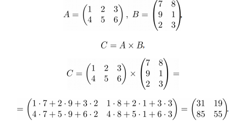
In Sympy, this is done through a simple multiplication operation.
A = Matrix([[1,2,3], [4,5,6]])
B = Matrix([[7,8], [9, 1], [2,3]])
C = A*B
In Numpy, this is done through the dot() operation:
A = np.array([[1,2,3], [4,5,6]])
B = np.array([[7,8], [9, 1], [2,3]])
C = A.dot(B)
print(C)
That’s all for today. In the next article, we will consider the solution of systems of linear equations, the methods of Gauss and Jordan, construction through decomposition and finding the determinant of a matrix. Write what else you want to know in my analysis. For personal communication with me: https://t.me/Nikotineaddiction