Linear Algebra for Data Science and Machine Learning
Linear algebra in Data Science and Machine Learning is foundational. Newbies starting their data science journey as well as established practitioners should develop a good understanding of the basic concepts of linear algebra.
Especially for the new start of the course Mathematics and Machine Learning for Data Science We share a translation of an article by Benjamin Obi Tayo – physicist, Ph.D., and Data Science educator – on what you need to know to better understand Data Science and Machine Learning.
Linear algebra is a branch of mathematics that is extremely useful in Data Science and Machine Learning. Linear algebra is also the most important math skill in machine learning. Most machine learning models can be expressed in matrix form. The dataset itself is often represented as a matrix. Linear algebra is used in data preprocessing, data transformation, and model evaluation. Here are the topics you should be familiar with:
Vectors.
Matrices.
Matrix transposition.
Inverse matrix.
Determinant of a matrix.
Matrix trace.
Scalar product.
Eigenvalues.
Own vectors.
In this article, we will illustrate the application of linear algebra in Data Science and Machine Learning using the technology stock market dataset that can be found here…
Linear algebra for data preprocessing
We’ll start by illustrating how linear algebra is applied to data preprocessing.
Importing Necessary Linear Algebra Libraries
import numpy as np
import pandas as pd
import pylab
import matplotlib.pyplot as plt
import seaborn as sns
Reading a dataset and displaying features
data = pd.read_csv("tech-stocks-04-2021.csv")
data.head()
print(data.shape)
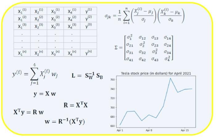
output = (11,5) The data.shape function lets us know the dimension of our dataset. In this case, the dataset contains 5 features (date, AAPL, TSLA, GOOGL and AMZN) and each contains 11 observations. Date refers to trading days in April 2021 (before April 16). AAPL, TSLA, GOOGL, and AMZN are the closing prices of Apple, Tesla, Google, and Amazon, respectively.
Data visualization
To visualize data, you need to define the columnar matrices of the visualized features:
x = data['date']
y = data['TSLA']
plt.plot(x,y)
plt.xticks(np.array([0,4,9]), ['Apr 1','Apr 8','Apr 15'])
plt.title('Tesla stock price (in dollars) for April 2021',size=14)
plt.show()
Covariance matrix
The covariance matrix is one of the most important matrices in Data Science and Machine Learning. It provides information about the joint movement (correlation) between features. Suppose we have a feature matrix with four signs and n observations as shown in Table 2:

To visualize the correlations between traits, we can generate a scatter plot:
cols=data.columns[1:5]
print(cols)
output = Index(['AAPL', 'TSLA', 'GOOGL', 'AMZN'], dtype="object")
sns.pairplot(data[cols], height=3.0)
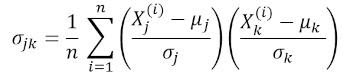
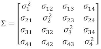
where μ and σ are the mean and standard deviation of the trait, respectively. This equation indicates that when features are normalized, the covariance matrix is simply the dot product between features. The covariance matrix can be expressed as a real and symmetric 4 x 4 matrix:
This matrix can be converted to a diagonal one by performing a unitary transformation, also called a principal component analysis (PCA) transformation, to get the following:
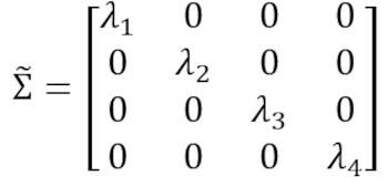
Since the trace of the matrix under the unitary transformation remains invariant, we observe that the sum of the eigenvalues of the diagonal matrix is equal to the total variance contained in the features Xone, X2, X3 and Xfour…
Computing the covariance matrix for technology stocks
from sklearn.preprocessing import StandardScaler
stdsc = StandardScaler()
X_std = stdsc.fit_transform(data[cols].iloc[:,range(0,4)].values)
cov_mat = np.cov(X_std.T, bias= True)
Note that this uses the transpose of the normalized matrix.
Visualization of the covariance matrix
plt.figure(figsize=(8,8))
sns.set(font_scale=1.2)
hm = sns.heatmap(cov_mat,
                 cbar=True,
                 annot=True,
                 square=True,
                 fmt=".2f",
                 annot_kws={'size': 12},
                 yticklabels=cols,
                 xticklabels=cols)
plt.title('Covariance matrix showing correlation coefficients')
plt.tight_layout()
plt.show()
Figure 3 shows that AAPL correlates strongly with GOOGL and AMZN and weakly correlates with TSLA. TSLA is usually weakly correlated with AAPL, GOOGL and AMZN, while AAPL, GOOGL and AMZN are highly correlated with each other.
Calculation of the eigenvalues of the covariance matrix
np.linalg.eigvals(cov_mat)
output = array([3.41582227, 0.4527295 , 0.02045092, 0.11099732])
np.sum(np.linalg.eigvals(cov_mat))
output = 4.000000000000006
np.trace(cov_mat)
output = 4.000000000000001
We observe that, as expected, the trace of the covariance matrix is equal to the sum of the eigenvalues.
Calculating Cumulative Variance
Since the trace of the matrix remains invariant under the unitary transformation, we observe that the sum of the eigenvalues of the diagonal matrix is equal to the total variance contained in the features Xone, X2, X3 and Xfour… Therefore, we can define the following quantities:

Please note that when p = 4, the cumulative variance becomes 1 as expected.
eigen = np.linalg.eigvals(cov_mat)
cum_var = eigen/np.sum(eigen)
print(cum_var)
output = [0.85395557 0.11318237 0.00511273 0.02774933]

print(np.sum(cum_var))
output = 1.0
From the cumulative variance (cum_var), we see that 85% of the variance is contained in the first eigenvalue and 11% in the second. This means that only the first two main components can be used in the PCA implementation, since 97% of the total variance is accounted for by these 2 components. This can significantly reduce the dimension of the feature space (from 4 to 2) when PCA is implemented.
Linear Regression Matrix
Suppose we have a dataset that has 4 predictor attributes and n observations as shown below.
")
We would like to build a multiple regression model to predict values y (column 5). Thus, our model can be expressed like this:
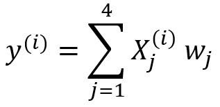
…
In matrix form, this equation can be written as follows:
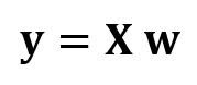
where X is a matrix of features (nx 4), w is a matrix (4 x 1) representing the regression coefficients being determined, and y is a matrix (nx 1) containing n observations of the target variable y.
Note that X is a rectangular matrix, so we cannot solve the above equation by taking the reciprocal of X.
To convert X to a square matrix, we multiply the left and right sides of our equation by the transposition from X, that is:
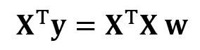
This equation can be written like this:
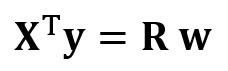
Where

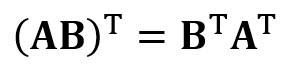
is a regression matrix (4 × 4). We observe that R is a real and symmetric matrix. Note that in linear algebra, the transposition of the product of two matrices obeys the following relationship:
Now that we have reduced our regression problem and expressed it in terms of a (4 × 4) real, symmetric, and invertible regression matrix R, it is easy to show that the exact solution to the regression equation looks like this:
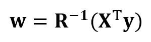
…
Examples of regression analysis for predicting continuous and discrete variables are given below:
The basics linear regression for absolute beginners.
Building perceptronic classifier using the least squares method.
Linear Discriminant Analysis Matrix
Another example of a real and symmetric matrix in Data Science is the Linear Discriminant Analysis (LDA) matrix. This matrix can be expressed like this:
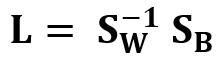
Where SW Is the within-feature scatter matrix, and SB – scattering matrix between features. Since both matrices SW and SB are real and symmetric, this implies that L is also real and symmetric. The diagonalization of L creates a feature subspace that optimizes class separation and dimensionality reduction. Therefore, LDA is a supervised learning algorithm, while PCA is not.
To learn more about the LDA implementation, please see the following links:
Machine Learning: dimensionality reduction using linear discriminant analysis.
Repository GitHub for an LDA implementation using the Iris dataset.
Python Machine Learning by Sebastian Raschka. 3rd ed. (chapter 5)…
Summary
So, we have discussed several applications of Linear Algebra in Data Science and Machine Learning. Using the tech stock market dataset, we illustrated important concepts such as matrix size, columnar matrices, square matrices, covariance matrices, matrix transposition, eigenvalues, dot products, etc.
Linear algebra is an essential tool in Data Science and Machine Learning. Thus, newcomers interested in Data Science should become familiar with the basic concepts of linear algebra.
To understand in detail the internal mechanics of Data Science, without disregarding machine learning, you can take a closer look at our course Mathematics and Machine Learning for Data Sciencewhere experienced mentors and experts in their field will answer difficult questions, eliminate ambiguities and correctly direct your thoughts, so that in the future you will solve difficult problems on your own.

find outhow to level up in other specialties or master them from scratch:
Other professions and courses
PROFESSION
COURSES