Introduction to Graph Neural Networks with a Self-Attention Mechanism Using PyTorch Geometric as an Example

To the start of the flagship data science course implement and compare a convolutional network and a network with a self-attention mechanism. Using t-SNE, we will show what and how is learned in a graph network with a self-attention mechanism. For details, we invite under cat.
Graph attention networks are, for obvious reasons, one of the most popular types of graph neural networks. In graph convolutional networks, all neighboring nodes have the same importance. It is obvious that this should not be the case.

This problem is solved in graph networks with an attention mechanism. To account for the importance of each neighbor node, a weighting factor is assigned to each connection by the attention mechanism.
Let’s calculate the weight coefficients and implement an efficient graph network with an attention mechanism in PyTorch Geometric. You can run the code for this tutorial at notepad Google Colab.
Graph Data

For our purposes, there are three classic graph datasets. These are networks of scientific papers, where each connection of nodes is a citation from a scientific work.
Cora. Consists of 2,708 machine learning papers in one of seven categories. Signs of the node – the presence (1) or absence (0) in the work of 1433 elements of the set of words. In other words, we are talking about a binary “bag of words”.
CiteSeer. A similar data set of 3312 scientific papers for classification into one of six categories. Signs of the node – the presence (1) or absence (0) in the work of elements of a set of 3703 words.
PubMed. This is a data set of 19,717 scientific publications on diabetes from the PubMed database in three categories. Node signs – weighted by TF-IDF word vectors from a dictionary of 500 unique words.
These datasets have been widely used in the scientific community. Using Multilayer Perceptrons (MLPs), Graph Convolutional Networks (GCNs), and Attentional Graph Networks (GATs), we compare our accuracy scores with those given in literature:

The PubMed dataset is quite large, and it will take longer to process and train a graph neural network on it. Cora is the most studied in the literature. Therefore, let’s take CiteSeer as an average option.
With a class planetoid In PyTorch Geometric, you can directly import any of these datasets:
from torch_geometric.datasets import Planetoid

# Import dataset from PyTorch Geometric
dataset = Planetoid(root=".", name="CiteSeer")

# Print information about the dataset
print(f'Number of graphs: {len(dataset)}')
print(f'Number of nodes: {dataset[0].x.shape[0]}')
print(f'Number of features: {dataset.num_features}')
print(f'Number of classes: {dataset.num_classes}')
print(f'Has isolated nodes: {dataset[0].has_isolated_nodes()}')
Number of graphs: 1
Number of nodes: 3327
Number of features: 3703
Number of classes: 6
Has isolated nodes: TrueWe have 3327 nodes instead of 3312. In fact, PyTorch Geometric uses the CiteSeer implementation from this work, which also shows 3327 nodes. But some of the nodes, namely 48, are isolated! It is not easy to classify them correctly without aggregation. Let’s plot the number of connections of each node using degree:
from torch_geometric.utils import degree
from collections import Counter

# Get list of degrees for each node
degrees = degree(data.edge_index[0]).numpy()

# Count the number of nodes for each degree
numbers = Counter(degrees)

# Bar plot
fig, ax = plt.subplots(figsize=(18, 7))
ax.set_xlabel('Node degree')
ax.set_ylabel('Number of nodes')
plt.bar(numbers.keys(),
        numbers.values(),
        color="#0A047A")
Most nodes only have 1 or 2 neighbors. This may explain CiteSeer’s lower accuracy scores than the other two datasets.
2. Self-attention
The term “self-attention” in graph neural networks first appeared in 2017 in the work Velickovic et al.when a simple idea was taken as a basis: not all nodes should have the same importance. And this is not just attention, but self-attention – here the input data is compared with each other:

By this mechanism, each connection is assigned a weighting factor (an indicator of attention). Let αᵢⱼ be the indicator of attention between nodes i and j. This is how the embedding of node 1 is calculated, where is the overall weight matrix:

But how do you calculate attention scores? You can write a static formula, but it makes more sense to find out their values using a neural network. The solution consists of these steps:
Linear transformation.
activation function.
Softmax normalization.
Linear transformation
To calculate the importance of each connection, pairs of hidden vectors are needed. The easiest way is to concatenate these vectors from both nodes. Only then can a new linear transformation be applied with the weight matrix ₐₜₜ:


Activation function
We are creating a neural network, so the second step is adding an activation function. In this case, the authors of the work chose the function LeakyReLU:


Softmax normalization
To compare indicators, the output of the neural network needs to be normalized. And to determine which node: 2 or 3 (α₁₂ > α₁₃), more important for node 1, nodes need the same scale. In neural networks, the softmax function is often used for this. Let’s apply it to each neighboring node:

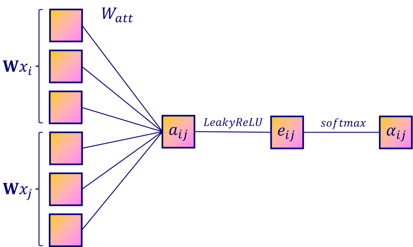
This is how each is calculated. αᵢⱼ. But self-attention is not very stable. To improve performance, the authors Vaswani et al. introduced the concept of “multi-headed attention” in the Transformer architecture.
Bonus: multi-headed attention
It’s amazing how much has been said about self-attention, even though Transformers are actually graph neural networks, so ideas from natural language processing apply here:

That is, in graph networks with an attention mechanism, multi-headed attention manifests itself in the repeated repetition of the same three stages in order to average or concatenate the results.
That’s all. Instead of one h₁ we get one hidden vector h₁ᵏ for each attention head. Then one of two schemes is applied:


In practice, the first scheme is applied on the output layer of the network, the second – on the hidden layer.
Graph attention networks
Implementing a graph network with an attention mechanism in PyTorch Geometric. This library has two graph attention layers: GATConv and GATv2Conv. So far, we have been talking about the first of them, but in 2021 Brody et al. improved by changing the order of operations.
The weight matrix is applied after the concatenation, and the attention weight matrix ₐₜₜ is applied after the LeakyReLU function. As a result, we have:


What layer to use? Brody et al. Gatv2Conv is said to consistently outperform GatConv.
And now let’s classify works from CiteSeer. I tried to roughly reproduce the experiments of the authors of the original, without unnecessarily complicating them. The official implementation of a graph network with an attention mechanism is on GitHub.
Graph attention layers are used in two configurations:
in the first layer, eight output neurons are concatenated – this is multi-headed attention;
in the second, there is only one head, and the final embeddings are calculated in it.
To compare accuracy scores, let’s train and test a graph convolutional network:
import torch.nn.functional as F
from torch.nn import Linear, Dropout
from torch_geometric.nn import GCNConv, GATv2Conv


class GCN(torch.nn.Module):
  """Graph Convolutional Network"""
  def __init__(self, dim_in, dim_h, dim_out):
    super().__init__()
    self.gcn1 = GCNConv(dim_in, dim_h)
    self.gcn2 = GCNConv(dim_h, dim_out)
    self.optimizer = torch.optim.Adam(self.parameters(),
                                      lr=0.01,
                                      weight_decay=5e-4)

  def forward(self, x, edge_index):
    h = F.dropout(x, p=0.5, training=self.training)
    h = self.gcn1(h, edge_index)
    h = torch.relu(h)
    h = F.dropout(h, p=0.5, training=self.training)
    h = self.gcn2(h, edge_index)
    return h, F.log_softmax(h, dim=1)


class GAT(torch.nn.Module):
  """Graph Attention Network"""
  def __init__(self, dim_in, dim_h, dim_out, heads=8):
    super().__init__()
    self.gat1 = GATv2Conv(dim_in, dim_h, heads=heads)
    self.gat2 = GATv2Conv(dim_h*heads, dim_out, heads=1)
    self.optimizer = torch.optim.Adam(self.parameters(),
                                      lr=0.005,
                                      weight_decay=5e-4)

  def forward(self, x, edge_index):
    h = F.dropout(x, p=0.6, training=self.training)
    h = self.gat1(x, edge_index)
    h = F.elu(h)
    h = F.dropout(h, p=0.6, training=self.training)
    h = self.gat2(h, edge_index)
    return h, F.log_softmax(h, dim=1)

def accuracy(pred_y, y):
    """Calculate accuracy."""
    return ((pred_y == y).sum() / len(y)).item()

def train(model, data):
    """Train a GNN model and return the trained model."""
    criterion = torch.nn.CrossEntropyLoss()
    optimizer = model.optimizer
    epochs = 200

    model.train()
    for epoch in range(epochs+1):
        # Training
        optimizer.zero_grad()
        _, out = model(data.x, data.edge_index)
        loss = criterion(out[data.train_mask], data.y[data.train_mask])
        acc = accuracy(out[data.train_mask].argmax(dim=1), data.y[data.train_mask])
        loss.backward()
        optimizer.step()

        # Validation
        val_loss = criterion(out[data.val_mask], data.y[data.val_mask])
        val_acc = accuracy(out[data.val_mask].argmax(dim=1), data.y[data.val_mask])

        # Print metrics every 10 epochs
        if(epoch % 10 == 0):
            print(f'Epoch {epoch:>3} | Train Loss: {loss:.3f} | Train Acc: '
                  f'{acc*100:>6.2f}% | Val Loss: {val_loss:.2f} | '
                  f'Val Acc: {val_acc*100:.2f}%')

    return model

def test(model, data):
    """Evaluate the model on test set and print the accuracy score."""
    model.eval()
    _, out = model(data.x, data.edge_index)
    acc = accuracy(out.argmax(dim=1)[data.test_mask], data.y[data.test_mask])
    return acc
%%time
# Create GCN
gcn = GCN(dataset.num_features, 16, dataset.num_classes)
print(gcn)
# Train
train(gcn, data)
# Test
acc = test(gcn, data)
print(f'GCN test accuracy: {acc*100:.2f}%\n')GCN(
(gcn1): GCNConv(3703, 16)
(gcn2): GCNConv(16, 6)
)
Epoch 0 | Train Loss: 1.782 | Train Acc: 20.83% | Val Loss: 1.79
Epoch 20 | Train Loss: 0.165 | Train Acc: 95.00% | Val Loss: 1.30
Epoch 40 | Train Loss: 0.069 | Train Acc: 99.17% | Val Loss: 1.66
Epoch 60 | Train Loss: 0.053 | Train Acc: 99.17% | Val Loss: 1.50
Epoch 80 | Train Loss: 0.054 | Train Acc: 100.00% | Val Loss: 1.67
Epoch 100 | Train Loss: 0.062 | Train Acc: 99.17% | Val Loss: 1.62
Epoch 120 | Train Loss: 0.043 | Train Acc: 100.00% | Val Loss: 1.66
Epoch 140 | Train Loss: 0.058 | Train Acc: 98.33% | Val Loss: 1.68
Epoch 160 | Train Loss: 0.037 | Train Acc: 100.00% | Val Loss: 1.44
Epoch 180 | Train Loss: 0.036 | Train Acc: 99.17% | Val Loss: 1.65
Epoch 200 | Train Loss: 0.093 | Train Acc: 95.83% | Val Loss: 1.73
GCN test accuracy: 67.70%
CPU times: user 25.1 s, sys: 847 ms, total: 25.9 s
Wall time: 32.4 s%%time
# Create GAT
gat = GAT(dataset.num_features, 8, dataset.num_classes)
print(gat)
# Train
train(gat, data)
# Test
acc = test(gat, data)
print(f'GAT test accuracy: {acc*100:.2f}%\n')GAT(
(gat1): GATv2Conv(3703, 8, heads=8)
(gat2): GATv2Conv(64, 6, heads=1)
)
Epoch 0 | Train Loss: 1.790 | Val Loss: 1.81 | Val Acc: 12.80%
Epoch 20 | Train Loss: 0.040 | Val Loss: 1.21 | Val Acc: 64.80%
Epoch 40 | Train Loss: 0.027 | Val Loss: 1.20 | Val Acc: 67.20%
Epoch 60 | Train Loss: 0.009 | Val Loss: 1.11 | Val Acc: 67.00%
Epoch 80 | Train Loss: 0.013 | Val Loss: 1.16 | Val Acc: 66.80%
Epoch 100 | Train Loss: 0.013 | Val Loss: 1.07 | Val Acc: 67.20%
Epoch 120 | Train Loss: 0.014 | Val Loss: 1.12 | Val Acc: 66.40%
Epoch 140 | Train Loss: 0.007 | Val Loss: 1.19 | Val Acc: 65.40%
Epoch 160 | Train Loss: 0.007 | Val Loss: 1.16 | Val Acc: 68.40%
Epoch 180 | Train Loss: 0.006 | Val Loss: 1.13 | Val Acc: 68.60%
Epoch 200 | Train Loss: 0.007 | Val Loss: 1.13 | Val Acc: 68.40%
GAT test accuracy: 70.00%
CPU times: user 53.4 s, sys: 2.68 s, total: 56.1 s
Wall time: 55.9 sThis experiment is not rigorous: it must be repeated n times and the final result should be the average accuracy with a standard deviation.
In this example, the attention network outperforms the convolutional network in accuracy (70.00% vs. 67.70), but it takes longer to train, i.e. 55.9 seconds vs. 32.4, which can cause scalability issues when working with large graphs.
The authors got 72.5% for the attentional network and 70.3% for the convolutional network, which is clearly better than our results. The difference can be explained by parameter settings in the models, as well as training settings (for example, patience 100 instead of a fixed number of epochs.
So, what did the network with the attention mechanism learn? We use a powerful method t-SNE for plotting high-dimensional data in 2D or 3D. First, let’s see what the embeddings looked like before training: as created from randomly initialized weight matrices, they should be completely random:
untrained_gat = GAT(dataset.num_features, 8, dataset.num_classes)

# Get embeddings
h, _ = untrained_gat(data.x, data.edge_index)

# Train TSNE
tsne = TSNE(n_components=2, learning_rate="auto",
         init="pca").fit_transform(h.detach())

# Plot TSNE
plt.figure(figsize=(10, 10))
plt.axis('off')
plt.scatter(tsne[:, 0], tsne[:, 1], s=50, c=data.y)
plt.show()
Indeed, there is no explicit structure here. But do embeds generated from a trained model look better?
h, _ = gat(data.x, data.edge_index)

# Train TSNE
tsne = TSNE(n_components=2, learning_rate="auto",
         init="pca").fit_transform(h.detach())

# Plot TSNE
plt.figure(figsize=(10, 10))
plt.axis('off')
plt.scatter(tsne[:, 0], tsne[:, 1], s=50, c=data.y)
plt.show()
The difference is noticeable: nodes of the same class are collected together. Six clusters are visible, corresponding to six classes of work. There are outliers, but that’s to be expected: our accuracy score is far from ideal.
Earlier, I suggested that nodes with bad connections can negatively affect the performance of CiteSeer. Calculate the accuracy of the model for each node connection:
from torch_geometric.utils import degree

# Get model's classifications
_, out = gat(data.x, data.edge_index)

# Calculate the degree of each node
degrees = degree(data.edge_index[0]).numpy()

# Store accuracy scores and sample sizes
accuracies = []
sizes = []

# Accuracy for degrees between 0 and 5
for i in range(0, 6):
  mask = np.where(degrees == i)[0]
  accuracies.append(accuracy(out.argmax(dim=1)[mask], data.y[mask]))
  sizes.append(len(mask))

# Accuracy for degrees > 5
mask = np.where(degrees > 5)[0]
accuracies.append(accuracy(out.argmax(dim=1)[mask], data.y[mask]))
sizes.append(len(mask))

# Bar plot
fig, ax = plt.subplots(figsize=(18, 9))
ax.set_xlabel('Node degree')
ax.set_ylabel('Accuracy score')
ax.set_facecolor('#EFEEEA')
plt.bar(['0','1','2','3','4','5','>5'],
        accuracies,
        color="#0A047A")
for i in range(0, 7):
    plt.text(i, accuracies[i], f'{accuracies[i]*100:.2f}%',
             ha="center", color="#0A047A")
for i in range(0, 7):
    plt.text(i, accuracies[i]//2, sizes[i],
             ha="center", color="white")
And the results confirm this assumption: nodes that have few neighbors are more difficult to classify. These are the features of graph neural networks: the more relevant connections, the more information is aggregated.
Conclusion
Although graph attention networks take longer to train, their accuracy is significantly higher than graph convolutional networks. Instead of static coefficients, the self-attention mechanism automatically calculates weight coefficients and embeddings are more accurate.
Graph attention networks are the de facto standard in many tasks using graph neural networks. However, longer training times can become a problem when working with large graph datasets. Scalability in deep learning is an important factor: usually a larger amount of data can lead to better performance.
And we will help you improve your skills or master a profession that is relevant at any time from the very beginning:
Choose another in-demand profession.

Brief catalog of courses and professions
Data Science and Machine Learning
Python, web development
Mobile development
Java and C#
From basics to depth
As well as


![Take and host your own LLM – why is it necessary? [и нужно ли вообще]](https://prog.world/wp-content/uploads/2024/06/6997ae04bd9f6ac6547282687f76d08b-768x428.jpg)