Do you think drawing lines is easy?

Take a ruler, pencil or pen and draw a line on the paper. You'll end up with something like this:

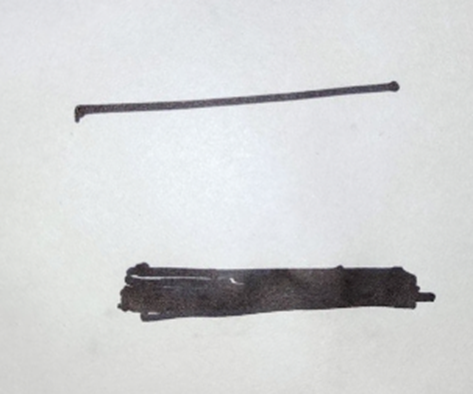
What's so difficult about drawing a line, you say? Now try using the same tool to draw a line 5-10 times the width of the point. It's more complicated isn't it?:

Okay, you say, I have a concealer that is much thicker than a pen! Yes, you will make things easier for yourself, but what if you need to draw a thicker line? It won't be easy again:

You will come to the conclusion that a thin line only seems thin; if you zoom in on it, you can see the width and error, as when drawing a line of greater width. But the whole point is that lines as a geometric object, i.e. a 1d object, are almost never found.

All lines that we can create have thickness, and lines with thickness are already defined planes (we will omit the fact that in our world everything has non-zero dimensions in all three planes). But since, most often, we need to have a uniform and symmetrical line, the line can be easily represented as a rectangle. This means that the task of drawing a line is reduced to the task of drawing a rectangle.

To visualize the process we will use OpenGL, namely geometry shaders in the GLSL language. All they do is take the points of the figure as input, and then build figures from them. All their code will be commented, so knowledge of GLSL is not required to understand the process.

To construct this rectangle, we know the coordinates of the centers of its sides located opposite each other. And also the width of these sides. We need to find the coordinates of the four corners of the rectangle.

Since the rectangle is symmetrical, this means that from the coordinates of one of the corners it will be possible to quite simply express the coordinates of the other corners.

Points P₀ And P₂ very similar to C₀ And C₁, however, they have displacements along the axes. Therefore, they can be expressed directly in terms of these offsets and point coordinates C₀ And C₁:

The coordinates of the points P₁ And P₂ it is even easier to obtain – through symmetry with respect to C₀ And C₁:

As a result, we only need to find the displacements x And y and through it it will be possible to obtain the coordinates of the remaining points. And this can be done in at least two different ways. The first requires minimal knowledge of geometry, the second requires knowledge of working with vectors. It’s up to you to decide which one is easier to understand, so I’ll describe both of them.

Method based on line length

Let's start with a method that requires only knowledge of the Pythagorean theorem. What is the essence of this method. We can get the distance to a point P₀ in two different ways, and from this we get two equations, solving which we get its coordinates. Subtracting the coordinates of the point from them C₀we will get this offset.

First, let's draw a picture:

We are interested in two straight lines L And M. Their length can be obtained using the source data like this:

Or through the point of interest to us like this:

Two equations, two variables, which means there is definitely a solution. All that remains is to find him. For the sake of rigor, I will give the complete stage of their solution, especially since it is trivial. Let's expand the brackets:

And one more:

Note that we can express the square of the length of the distance between the starting points:

As a result we get:

And thanks to this, you can simplify the expression a little:

Now we can equate both parts:

Let's remove repetitions and combine identical variables, at the same time changing the signs:

Let's express x And y through each other:

Let's substitute into the original equation:

Let's bring it to zero:

Let's solve it for x:

Likewise, for y:

They can also be simplified, for this we will open the brackets:

Note that the square root is the modulus, and the divisor is the distance between the starting points:

In general, since each expression has two solutions that differ only in sign, and S And L are always positive, the module can be removed:

As a result, we received two equations; the only question that remains is which of the two solutions to each equation corresponds to our shift relative to the original points.

To do this, consider the four positions of the rectangle-line in space, relative to the center. Since the points are symmetrical, as was shown earlier, we will show the effect only on the point P₀ :

Since the sign is affected only by the difference between the coordinates of the original points, we analyze their signs in all possible positions of the point P₀:

As can be seen from the table, the offset for y exactly advises the sign of the difference in coordinates, which means the equation for the displacement y will have a positive sign for the point P₀ (and for the point P₁ due to symmetry, negative sign).

For x the situation is exactly the opposite, the sign of the displacement is always different than the sign of the difference, which means the equation for the displacement x will have a negative sign for the point P₀ (and for the point P₁ due to symmetry, the sign is positive).

As a result, we finally get the offset:

The next method will lead us to the same result, but in a completely different way…

Orthogonality based method

Points on a plane can be represented as vectors showing directions and speed (their length) from the origin. Then, let the points P₀ ,C₀ And C₁ this is a vector P₀^–,C₀^– And C₁^– directed from the origin.

This method is based on the fact that P₀^– And C₀^– orthogonal (i.e., there is an angle of 90 degrees between them). This means we can rotate the vector obtained from the difference of vectors C₀^– And C₁^– by 90 degrees and get a vector C₂^– the same length as the distance from C₀^– before C₁^–. We also know the distance from P₀^– before C₀^– . Therefore, to determine the vector P₀^– it is enough to find the ratio of the vector lengths and multiply the coordinates by it C₂^– . And already through the coordinates P₀^– find the offset.

First, let's find the difference vector C₀^– And C₁^–:

For the resulting vector C₂^– We use the formula for rotating a vector by an angle on a plane:

Let's substitute 90 degrees into the formula to make it orthogonal to the vector P₀^– get the codirectional vector:

As a result, we obtain the following definition of point coordinates:

Next, we find the ratio of vector lengths C₂^– and given width S:

All that remains is to change the vector length C₂^– without changing its direction, to do this we multiply its coordinates by the length ratio:

Let's put it in place TO his equation:

We again came to the same formulas as last time!

Visualization of the result

And now we have everything we need to draw a line. Now let's visualize this, putting everything together at the same time. To do this, we need a rendering pipeline, which consists of 6 stages. Each of which processes its own data (more details in this series of articles). Of these, we can influence only three stages (highlighted in blue):

For our case, the vertex shader simply rearranges the vertices, moving them into the vertex shader. The model matrix is ​​needed to position the entire line in space (more details):

#version 330 core

//координаты точек линии
layout (location = 0) in float position_x;
layout (location = 1) in float position_y;

//матрица модели, задающая положения  объекта в пространстве
uniform mat4 model;

void main(){
   //передача позиции точек в геометрический шейдер
    gl_Position = model *vec4(position_x,position_y,0.0f,1.0f);
}

The fragment shader is even simpler, it sets one color for the entire line:

#version 330 core

out vec4 color;
uniform  vec4 mat_color;

void main(){
    color=mat_color;//передаём цвет в растеризатор
};

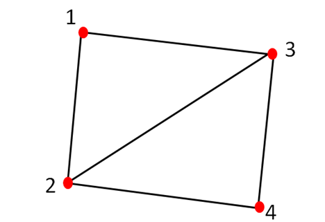
Any 2d objects can be represented as a group of triangles (with some error, of course). So we will draw a line using them. The geometry shader receives two points (a line segment) and based on them constructs a rectangle from two triangles. Since output from a geometry shader is only possible in the form triangle_strip (each vertex after the second creates a new triangle), the vertices will be presented in this order:

The geometry shader code itself:

#version 400 core
layout (lines) in;//входные данные, две точки (x0;y0) и (x1;y1)

//входные данные, точки прямоугольника
//(прямоугольник рисуется с помощью двух треугольников,
//strip значит, что для построения второго треугольника 
//будут использованны две вершины предыдущего)
layout (triangle_strip, max_vertices = 4) out;

in  float S[];//передаём ширину линии

//Функция определения смещения
vec2 get_general_point_corner(vec2 P0,vec2 P1){
    float L =(distance(P0,P1));

    float K=S[0]/L;

    float x_=-K*(P1.y-P0.y);
    float y_=K*(P1.x-P0.x);

    return vec2(x_,y_);
}

void bild_quard(vec2 A_0, vec2 P0, vec2 P1){
    // 1:bottom-left
    gl_Position =vec4((A_0.x+P0.x), (A_0.y+P0.y), 0.0, 1.0);    
    EmitVertex();
    // 2:bottom-right
    gl_Position =vec4((-A_0.x+P0.x),  (-A_0.y+P0.y), 0.0, 1.0);    
    EmitVertex();
    // 3:top-left
    gl_Position =vec4((A_0.x+P1.x), (A_0.y+P1.y), 0.0, 1.0);    
    EmitVertex();
    // 4:top-right
    gl_Position =vec4((-A_0.x+P1.x),  (-A_0.y+P1.y), 0.0, 1.0);  
    EmitVertex();
}

void main() {
    //получаем смещения
    vec2 p_= get_general_point_corner(gl_in[0].gl_Position.xy,gl_in[1].gl_Position.xy);
    //строим прямоугольник-линию
    bild_quard(p_,gl_in[0].gl_Position.xy,gl_in[1].gl_Position.xy);
    EndPrimitive();
}

As a result, we get the following:

The problem of the junction of two lines

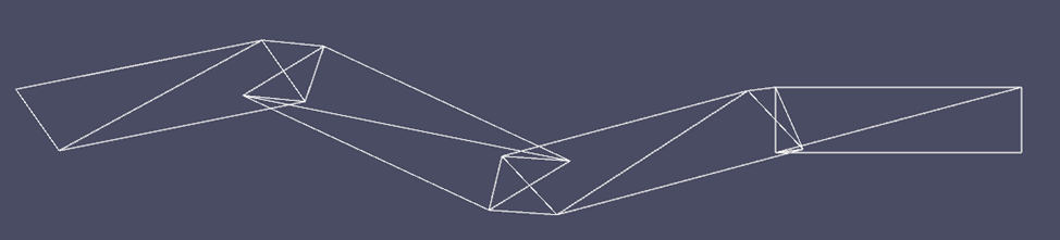
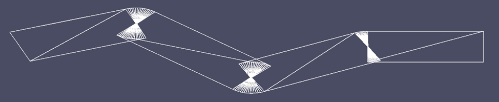
Everything is fine with one line, let's try to draw a curve from different lines:

As we can see, there is a problem at the junction of the segments – they are not connected, you need to separately implement the connection of the lines. In principle, three types of connections can be distinguished:

• Oblique

• Direct

• Rounded

To implement each of them, we will need information about the vertices of other segments. For this instead layout (lines) in in the shader we use layout (lines_adjacency) in, which gives information about the vertices of other segments.

Oblique connection

Overall we can just connect the dots P₂ And P₄ in the following way:

To do this, we get the offset for another rectangle in the geometry shader, and find the point through it P₄. It would be possible to figure out exactly which side to draw the triangle for a smooth junction based on the slope of the two lines, but it is better to draw an extra triangle than to add a condition. To do this, let's find a point P₅ and draw a rectangle P₂P₄P₃P₅.

The division of its vertices into triangles will be the same:

The shader code, based on the above, will look like this:

#version 400 core
//входные данные, четыре точки (x0;y0),(x1;y1),(x2;y2) и (x3;y4)
layout (lines_adjacency) in;

//входные данные, точки прямоугольника
//(прямоугольник рисуется с помощью двух треугольников,
//strip значит, что для построения второго треугольника 
//будут использованны две вершины предыдущего)
layout (triangle_strip, max_vertices = 6) out;

in  float S[];//передаём ширину линии

//Функция определения смешения
vec2 get_general_point_corner(vec2 P0,vec2 P1){
    float L =(distance(P0,P1));

    float K=S[0]/L;

    float x_=-K*(P1.y-P0.y);
    float y_=K*(P1.x-P0.x);

    return vec2(x_,y_);
}


void bild_quard(vec2 A_0, vec2 P0, vec2 P1){
    // 1:bottom-left
    gl_Position =vec4((A_0.x+P0.x), (A_0.y+P0.y), 0.0, 1.0);    
    EmitVertex();
    // 2:bottom-right
    gl_Position =vec4((-A_0.x+P0.x),  (-A_0.y+P0.y), 0.0, 1.0);    
    EmitVertex();
    // 3:top-left
    gl_Position =vec4((A_0.x+P1.x), (A_0.y+P1.y), 0.0, 1.0);    
    EmitVertex();
    // 4:top-right
    gl_Position =vec4((-A_0.x+P1.x),  (-A_0.y+P1.y), 0.0, 1.0);  
    EmitVertex();
}

void oblique_connection(vec2 A_1, vec2 P1){
    // верхний треугольник в стыке
    gl_Position =vec4((A_1.x+P1.x), (A_1.y+P1.y), 0.0, 1.0);       
    EmitVertex();
    // нижний треугольник в стыке
    gl_Position =vec4((-A_1.x+P1.x), (-A_1.y+P1.y), 0.0, 1.0);       
    EmitVertex();
}

void main() {
    //получаем смещения
    vec2 p_= get_general_point_corner(gl_in[0].gl_Position.xy,gl_in[1].gl_Position.xy);
    vec2 p_1=get_general_point_corner(gl_in[1].gl_Position.xy,gl_in[2].gl_Position.xy);
     //строим прямоугольник-линию
    bild_quard(p_,gl_in[0].gl_Position.xy,gl_in[1].gl_Position.xy);
   
    //строим соединение стыка линий
    oblique_connection(p_1,gl_in[1].gl_Position.xy);
    EndPrimitive();
}

In the end it will look like this:

This is the most effective method in terms of the number of triangles and the description of the method. However, other solutions to this problem are possible.

Direct connection

For this type of joint resolution, we need to define a point P₆ :

Fortunately, this is very easy to do, since our line segments are on the same plane, you can always find the intersection point of two straight lines or say that they are parallel. This means that in order to find this point, we must find by points P₀ And P₂ the first equation of a straight line, and by points P₄ And P₅ second equation, and then equate them.

First, let's write the equation of a straight line through two points for P₀ And P₂ :

Let's rewrite it through the offsets and coordinates of the original points of the line (i.e., centers), for this we simply expand the variables:

The result is a terrible equation:

Let's cut down the unnecessary ones:

Let's expand the brackets:

Let's simplify it again:

Let's divide it into three parts:

Multiply the first and second parts by S/L :

Let's change the signs in brackets:

And let's simplify it finally:

Let's rewrite parts of the equation as individual constants:

Then the equation will take the form:

Why did we do this?

First, we got two constant components. First, c shows the displacement relative to the coordinate center to the center of the central line (looking at the equation of the line through two points, we will see exactly the same constant, which will be the only one that shows the displacement).

Secondly, b shows the offset from the center line of the rectangle to the boundaries. The sign indicates on which side the straight line given by the equation is located, on the left (‑) or on the right (+).

Next, we equate the equation:

And we find the coordinate x (y can be found through any other equation):

As mentioned in the bevel method, using conditionals in the shader can be less efficient than adding more triangles. Therefore, we will additionally find the intersection point through straight lines laid through the other two sides of the rectangle. Fortunately, this is just a change in the sign of the variable b to the opposite, according to the second fact.

We will draw triangles for this joint in this order, because of the requirement, each point after the second is a new triangle. And here, in any case, we will have to build additional points, even if we take into account the direction of the bevel, so we will build it in a mirror way, placing the vertices like this:

I think there is no need to explain the shader code, everything here is also quite simple. The only new thing is the function that determines the position of the point P₆ (P₉ ):

#version 400 core
//входные данные, четыре точки (x0;y0),(x1;y1),(x2;y2) и (x3;y4)
layout (lines_adjacency) in;

//входные данные, точки прямоугольника
//(прямоугольник рисуется с помощью двух треугольников,
//strip значит, что для построения второго треугольника 
//будут использованны две вершины предыдущего)
layout (triangle_strip, max_vertices = 6) out;

in  float S[];//передаём ширину линии

//Функция определения смешения
vec2 get_general_point_corner(vec2 P0,vec2 P1){
    float L =(distance(P0,P1));

    float K=S[0]/L;

    float x_=-K*(P1.y-P0.y);
    float y_=K*(P1.x-P0.x);

    return vec2(x_,y_);
}


void bild_quard(vec2 A_0, vec2 P0, vec2 P1){
    // 1:bottom-left
    gl_Position =vec4((A_0.x+P0.x), (A_0.y+P0.y), 0.0, 1.0);    
    EmitVertex();
    // 2:bottom-right
    gl_Position =vec4((-A_0.x+P0.x),  (-A_0.y+P0.y), 0.0, 1.0);    
    EmitVertex();
    // 3:top-left
    gl_Position =vec4((A_0.x+P1.x), (A_0.y+P1.y), 0.0, 1.0);    
    EmitVertex();
    // 4:top-right
    gl_Position =vec4((-A_0.x+P1.x),  (-A_0.y+P1.y), 0.0, 1.0);  
    EmitVertex();
}

vec2 get_point_corner(int side,
                      vec2 A_0,vec2 P0,vec2 P1,
                      vec2 A_1,vec2 P2,vec2 P3){

    float a_0= -A_0.x/A_0.y;
    float a_1= -A_1.x/A_1.y;

    float b_0 = side*(A_0.x*A_0.x+A_0.y*A_0.y)/A_0.y + (P1.x*P0.y-P0.x*P1.y)/(P1.x-P0.x);
    float b_1 = side*(A_1.x*A_1.x+A_1.y*A_1.y)/A_1.y + (P3.x*P2.y-P2.x*P3.y)/(P3.x-P2.x);

    float x=-(b_0-b_1)/(a_0-a_1);
    float y=a_0*x+b_0;

    return vec2(x,y);
}

void direct_connection(vec2 T_0, vec2 T_1,vec2 A_1, vec2 P1){
    gl_Position =vec4(T_0.xy, 0.0, 1.0);
    EmitVertex();
    gl_Position =vec4(T_1.xy, 0.0, 1.0);
    EmitVertex();
    gl_Position =vec4((A_1.x+P1.x), (A_1.y+P1.y), 0.0, 1.0);
    EmitVertex();
    gl_Position =vec4((-A_1.x+P1.x), (-A_1.y+P1.y), 0.0, 1.0);
    EmitVertex();
}

void main() {
    //получаем смещения
    vec2 p_= get_general_point_corner(gl_in[0].gl_Position.xy,gl_in[1].gl_Position.xy);
    vec2 p_1=get_general_point_corner(gl_in[1].gl_Position.xy,gl_in[2].gl_Position.xy);

    //ищём точку угла
    vec2 t_= get_point_corner( 1,p_,gl_in[0].gl_Position.xy,gl_in[1].gl_Position.xy,                 
                                                  p_1,gl_in[1].gl_Position.xy,gl_in[2].gl_Position.xy);
    vec2 t_1=get_point_corner(-1,p_,gl_in[0].gl_Position.xy,gl_in[1].gl_Position.xy,                    
                                      p_1,gl_in[1].gl_Position.xy,gl_in[2].gl_Position.xy);

     //строим прямоугольник-линию
    bild_quard(p_,gl_in[0].gl_Position.xy,gl_in[1].gl_Position.xy);

   
    //строим соединение стыка линий
    direct_connection(t_,t_1,p_1,gl_in[1].gl_Position.xy);
    EndPrimitive();
}

As a result, we will see on the screen:

Already better than the previous method, and quite a good result. But you can do something even more interesting and round the line.

Round connection

In the previous method, we defined the points for the straight joint. And in the skew joint method, we used points on different lines to create a skew line. In this method, we will need all three points to use a square Bezier curve (more details in an excellent article). This method is intermediate between both joints.

To draw this curve we need its equation:

where t is in the range 0 to 1.

It is enough to change t with a certain step, which will determine the bending accuracy (the larger the step, the less accuracy). Here you will also need to mirror the points for convenient drawing of points:

As you can see, to draw such a paired bend, it is enough to add points from both lines in turn. The shader for rendering this case is based on this:.

#version 400 core
//входные данные, четыре точки (x0;y0),(x1;y1),(x2;y2) и (x3;y4)
layout (lines_adjacency) in;

//входные данные, точки прямоугольника
//(прямоугольник рисуется с помощью двух треугольников,
//strip значит, что для построения второго треугольника 
//будут использованны две вершины предыдущего)
layout (triangle_strip, max_vertices = 48) out;

in  float S[];//передаём ширину линии

//Функция определения смешения
vec2 get_general_point_corner(vec2 P0,vec2 P1){
    float L =(distance(P0,P1));

    float K=S[0]/L;

    float x_=-K*(P1.y-P0.y);
    float y_=K*(P1.x-P0.x);

    return vec2(x_,y_);
}


void bild_quard(vec2 A_0, vec2 P0, vec2 P1){
    // 1:bottom-left
    gl_Position =vec4((A_0.x+P0.x), (A_0.y+P0.y), 0.0, 1.0);    
    EmitVertex();
    // 2:bottom-right
    gl_Position =vec4((-A_0.x+P0.x),  (-A_0.y+P0.y), 0.0, 1.0);    
    EmitVertex();
    // 3:top-left
    gl_Position =vec4((A_0.x+P1.x), (A_0.y+P1.y), 0.0, 1.0);    
    EmitVertex();
    // 4:top-right
    gl_Position =vec4((-A_0.x+P1.x),  (-A_0.y+P1.y), 0.0, 1.0);  
    EmitVertex();
}

vec2 get_point_corner(int side,
                      vec2 A_0,vec2 P0,vec2 P1,
                      vec2 A_1,vec2 P2,vec2 P3){

    float a_0= -A_0.x/A_0.y;
    float a_1= -A_1.x/A_1.y;

    float b_0 = side*(A_0.x*A_0.x+A_0.y*A_0.y)/A_0.y + (P1.x*P0.y-P0.x*P1.y)/(P1.x-P0.x);
    float b_1 = side*(A_1.x*A_1.x+A_1.y*A_1.y)/A_1.y + (P3.x*P2.y-P2.x*P3.y)/(P3.x-P2.x);

    float x=-(b_0-b_1)/(a_0-a_1);
    float y=a_0*x+b_0;

    return vec2(x,y);
}

void bezier_connection(vec2 T_0, vec2 T_1,vec2 A_0,vec2 A_1, vec2 P1){
    vec2 H0=vec2( A_0.x+P1.x, A_0.y+P1.y);
    vec2 H1=vec2(-A_0.x+P1.x,-A_0.y+P1.y);

    vec2 H2=vec2( A_1.x+P1.x, A_1.y+P1.y);
    vec2 H3=vec2(-A_1.x+P1.x,-A_1.y+P1.y);

    float t=0.0;
    int count=16;
    for(int z = 0; z < count+1; z++){
        vec2 B_0=(1-t)*(1-t)*H0+2*t*(1-t)*T_0+t*t*H2;
        vec2 B_1=(1-t)*(1-t)*H1+2*t*(1-t)*T_1+t*t*H3;

        gl_Position =vec4(B_0.xy, 0.0, 1.0);
        EmitVertex();
        gl_Position =vec4(B_1.xy, 0.0, 1.0);
        EmitVertex();

        t+=1.0/count;
    }
}


void main() {
    //получаем смещения
    vec2 p_= get_general_point_corner(gl_in[0].gl_Position.xy,gl_in[1].gl_Position.xy);
    vec2 p_1=get_general_point_corner(gl_in[1].gl_Position.xy,gl_in[2].gl_Position.xy);

    //ищём точку угла
    vec2 t_= get_point_corner( 1,p_,gl_in[0].gl_Position.xy,gl_in[1].gl_Position.xy,                 
                                                  p_1,gl_in[1].gl_Position.xy,gl_in[2].gl_Position.xy);
    vec2 t_1=get_point_corner(-1,p_,gl_in[0].gl_Position.xy,gl_in[1].gl_Position.xy,                    
                                      p_1,gl_in[1].gl_Position.xy,gl_in[2].gl_Position.xy);

     //строим прямоугольник-линию
    bild_quard(p_,gl_in[0].gl_Position.xy,gl_in[1].gl_Position.xy);
   
   //строим соединение cтыка линий
    bezier_connection(t_,t_1,p_,p_1,gl_in[1].gl_Position.xy);
    EndPrimitive();
}

And in the end we get:

As you can see, each subsequent joining method also uses intermediate calculations of the previous one, which clearly shows why this particular order of description of methods was chosen.

Instead of a conclusion

There are many things in our life that at first glance seem simple, for example, a line. But if you take a closer look, everything becomes much more interesting. Even to draw a simple line, slightly thicker than a tool, we need to remember the basics of geometry.

Answering the question posed in the title of the article, we can say that drawing lines is easy if they are thin, but difficult if the eye can see the differences.