Derivative with real exponent

This idea was shared with me by a classmate in the Physics Department of Kharkov University, Vitka Serednitsky, at one of the communal gatherings (read – drinking bouts). We were young, diligently gnawed at the granite of science, seriously thought that we would be engaged in theoretical physics all our lives, and the time for dreams was right in the yard – the year was about 1989. The idea turned out to be not new, but I got excited to explore it, and that’s what happened.

A well-behaved function (I skip the math here) can be represented as a Fourier series, a sine and cosine expansion:

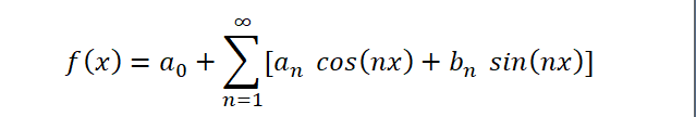
(we take, for simplicity, the interval [–π, π ]in order not to write out additional coefficients of the form π/l)

Since sines and cosines are periodic functions, the expanded function also turns into a periodic one. For function y=x on the entire numerical axis, its graph will look like this, piecewise:

You can expand the range with [–π, π] to any [–l, l]and even aiming l to infinity, turn the series into an integral so that the expansion becomes applicable to the entire number line. We will not deal with this, for the purpose of our article it is not essential.

The coefficients of the Fourier series are determined by the formulas, n = 0, 1, 2, 3..

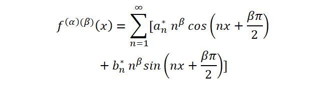
Further, the series, under certain conditions of its convergence, can be differentiated term by term, then we obtain for the first derivative

Vitya noticed that the transformation of a sine into a cosine and vice versa is equivalent to a shift by π/2and then the last formula can be written as:

Well, now it remains only to postulate for a derivative with a real exponent α

The “zero” derivative will coincide with the original function itself, with α = 1 we get the usual first derivative.

(Derivatives – I have seen such a designation – are written as a degree in parentheses, if you do not use the “single number system” with the required number of strokes. However, in this case, for some reason, the derivative exponent was denoted by a Roman numeral! How to write real numbers in Roman numerals, I just don’t represent).

Let’s explore this definition.

First, I wonder if the order of differentiation affects the result. Let us take successively the derivative with alpha and then with beta. The calculation procedure – there are quite simple algebraic transformations – we will remove it under the cat, the result is positive:

Under the cut

We expand the cosine and sine of the sum in the formula for the derivative of order alpha, regroup the terms, and reduce to the form of the usual Fourier expansion

Where

Now again we apply the formula for the derivative of order β

If we now substitute here the expressions for a*_n and b*_n and then roll back the resulting terms into the cosine and sine of the sum of the angles, we finally get

Now let’s touch on convergence. The usual convergence of the series at each point is beyond doubt. The issue is uniform convergence. The amazing thing is that I managed to prove it only for even functions (symmetric about the axis Y), otherwise, it seems that it does not take place, a little later we will see indirect confirmation of this.

It is interesting that the concept of uniform convergence appeared (well, or was realized) quite late. In general, it must be said that finally all the subtle questions of mathematical analysis were clarified and completed only by the middle of the 19th century, almost 200 years after its creation by the geniuses Newton and Leibniz. In terms of uniform convergence, this merit belongs to Karl Weierstrass (Wikipedia articleit’s better to watch more complete English version).

And finally, let’s move on to the charts.

Pants are turning… Pants are turning…

The simplest linear function becomes a constant, not without difficulty:

The parabola smoothly transforms into a linear function:

Cubic parabola becomes quadratic

The graph turned out to be very cluttered, let’s expand it:

The exponent, after some fluctuations, again merges with itself:

Hyperbolic cosine becomes hyperbolic sine

(By the way, how did you shortly call hyperbolic functions? We have “shinus” and “chosine”)

It can be seen that even functions (x², ch(x)) the convergence goes smoothly, and the odd ones with beats, which confirms the thesis about the absence of uniform convergence in the general case. We note here that the hyperbolic cosine (“chosine”) is nothing more than the selection of its even part from the exponent – according to the well-known formula for dividing any function into even and odd:

– and we immediately obtain uniform convergence for the even part (at least “by eye”).

It’s a shame that not all elementary functions make it possible to obtain the formula of the Fourier coefficients in an analytical form – neither for the natural logarithm, nor for a function of type 1/x, this is possible. It would be possible, of course, to count them programmatically, but it seemed to me that the examples given are quite enough, the high-quality picture is approximately the same for different functions.

Orthogonal systems of functions

A bit about expanding functions into series. An amazing thing, but the simplest, elementary expansion of a vector on a plane along two guides along the axes X And Y can be extended far to the case of functions. Let’s say we have an ordinary vector space R² with the operations of adding vectors and multiplying a vector by a number. The decomposition of a vector in an ordinary Cartesian space can also be introduced through the notion of a dot product.

For vectors a = (a_xa_y) b = (b_x,b_y) their dot product is defined as

= a_x*b_x+a_y*b_y

If the product is zero, the vectors are orthogonal. In other cases, we get the projection of one vector onto the direction of another. The scalar product of a vector with itself gives just the square of its length – by the Pythagorean theorem

<a, a>=a_x² + a_y²

Consider 2 vectors (orts) of the form n_x = (1,0) and n_y= (0,1). They are orthogonal <n_x, n_y> = 0 and normalized to unity <n_x,n_x>=<n_y,n_y>=1

The product of the orth by any vector is the projection of the vector onto the corresponding axis:

<a, n_x>=a_x <a, n_y>=a_y

And any vector in R² imagine how

a =<a, n_x>n_x +<a, n_y>n_y,

i.e. the vector n_x And n_y form a basis.

The function space can also be declared a linear vector space. And if we come up with an scalar product in this space, then all the above considerations and conclusions can be safely transferred here – although in this case it is not at all obvious what can be understood, for example, as “the square of the length of a function”, “the angle between two functions”, or “ orthogonality of two functions to each other. The latter simply means that their scalar product is equal to zero.

The scalar product in the space of functions can be introduced as follows:

And the vectors of such a space (it is called L²) we declare all functions for which such an integral is finite on any bounded interval (that is, any function has a specific finite “length”, whatever that means). Then the scalar product of any two functions from L² – of course (according to the Cauchy-Bunyakovsky-Schwartz inequality).

And, as it turns out, in this space there is an infinite basis of mutually orthogonal functions of the form sin(nx), cos(nx), because the

And the same for the product of sines, and for the product of sine and cosine there will always be zero.

Now it immediately becomes clear where the formulas for the coefficients come from a_n, b_n at the beginning of the article (these are simply “projections” of the function onto the corresponding vector from the basis, chbenz), and the Fourier series itself.

(we do not touch here on the convergence of such infinite expansions in general, the convergence to our function, as well as other subtle issues, but only the conceptual part)

It turns out that sines and cosines are not the only possible basis in the space of functions! There are other systems of orthogonal functions, such as the Legendre polynomials. Interestingly, the Gram-Schmidt orthogonalization process for the usual series of power functions leads to these polynomials − 1, x, x², x³). And the expansion in the Taylor series, in which, as we know, all infinitely differentiable functions decompose, can be translated into an expansion in Legendre polynomials. Details here.

Reasoning non-mathematician.

Let’s try this line of reasoning. If the property of some mathematical object is expressed, for example, by a natural number, then why not imagine that there can be objects in which this property is an integer (that is, it can be zero or negative), fractional (rational), real, and so on ? The main thing is that in already known situations, the definition of such a property coincides with the original one, and then there is room for interpolations. In the end, the same Pythagoreans believed that the numbers themselves can only be natural, the rest is from the evil one, and as a result, the concept of a real number and continuum was delayed until the very end of the 19th century.

It is unlikely that mathematical discoveries are made in such a “mechanical” way. However, we can offhand name several areas where, in fact, such a generalization happened:

– degree with a real indicator – through natural logarithms,

– complex numbers (“who said that you can’t take roots from negative numbers”?),

– distances between points in pseudo-Euclidean space, which can be negative – and it’s amazing how this has found application in the Special Theory of Relativity,

– fractional dimension of topological spaces and all sorts of tricky sets

Well, etc. and so on. A derivative with a real exponent also fits well in this series. Are there any other examples? – write in the comments!

Hello, ~~Andrey~~ Ptolemy!

Interestingly, the system of epicycles and deferents of Ptolemy, which tried to explain the motions of the planets incomprehensible to the ancients, was, in fact, the same expansion in a Fourier series, perhaps in a slightly distorted form. Were we to produce a sufficient number of such circles, along which conditional points revolve around the Earth, and around them – more points, the centers of other circles, it would be possible to approach the true movements of the planets with arbitrarily accurate, and no system of the world of Copernicus with the Sun in the center can would need!