testing and monitoring of the user negativity model

Hello! On the line Alexey, Alexander And Alice. In the previous article We looked at the technical aspects of training an ML algorithm to predict user rejection of advertising.
The model identifies users who should not be bothered with advertising communications today, which reduces the dynamics of user refusals from marketing while maintaining the overall level of product activity.
In this article, we will consider the metrics used to monitor the quality of the model and assess its accuracy in production. We will talk about measuring the statistically significant efficiency of the solution obtained using the fixed horizon a/b test. We will consider the consistent use of statistical criteria using the ratio metric as an example.
Comparison of quality metrics: training dataset vs real business process.
Let's look at the distribution of model scores, ROC curves, and Precision-Recall vs. Threshold curves built on a sampled training dataset and on real data.
")
")
The appearance of the histogram of the distribution of scores has remained virtually unchanged, but we see a decrease in the ROC AUC metric and a strong drop in the accuracy of the algorithm – Precision.
Real data is very different from sampled data: sampled examples conversion to marketing abandonment was about 5%, but in real data, our bad rate was 293 clients with refusals among 10,980,642 active ones per day, that is, ≈ 2.67e-5.
The absolute value of precision is extremely small due to the large number of False Positive (FP) examples. Strictly speaking, with such an imbalance of classes, the ROC_AUC metric is insensitive and will show a relatively good result.
Let us give an illustrative example.
Confusion matrix | |||
Real values of classes (y) | |||
y = 1 | y = 0 | ||
Algorithm predictions (ŷ) | ŷ = 1 | True Positive (TP) | False Positive(FP) |
ŷ = 0 | False Negative (FN) | True Negative (TN) | |
Let's assume that we need to find one hundred special examples out of one million. Let's agree that the data is prepared correctly, there is no noise and duplicates.
Let's consider two algorithms.
Algorithm 1 | Algorithm 2 |
Returns 100 responses, of which: 90 – True Positive (TP) guessed correctly; 10 – incorrect False Positive (FP). In this case, FN = 10 (there are 100 special examples in total, the algorithm found 90, which means that 10 of them are FN). In this case, TN = 999,890 (a total of 999,900 “0-examples”, the algorithm identified 10 examples incorrectly as special) | Returns 2000 responses, of which: 90 – True Positive (TP) guessed correctly; 1910 – incorrect False Positive (FP). In this case, FN = 10 (there are 100 special examples in total, the algorithm found 90, which means that 10 of them are FN). In this case, TN = 997,990 (a total of 999,900 “0-examples”, the algorithm incorrectly identified 1,910 examples as special) |
Let's calculate ROC_AUC for binary response — “fair accuracy” in a problem with class imbalance | |
TPR = TP / (TP + FN) = 90 / (90 + 10) = 0.9 FPR = F / (FP + TN) = 10 / (10 + 999,890) ≈ 1e-5 ROC_AUC = (1 + 0.9 − 0.00001) / 2 = 0.949995 | TPR = TP / (TP + FN) = 90 / (90 + 10) = 0.9 FPR = FP / (FP + TN) = 1910 / (1,910 + 997,990) ≈ 191e-5 ROC_AUC = (1 + 0.9 − 0.00191) / 2 = 0.949045 |
That is, ROC_AUC differs only in the fourth decimal place! Let's look at Recall and Precision.
Algorithm 1 | Algorithm 2 |
Recall = TP / (TP + FN) = 0.9 / (90 + 10) = 0.9 Precision = TP / (TP + FP) = 90 / (90 + 10) = 0.9 | Recall = TP / (TP + FN) = 0.9 / (90 + 10) = 0.9 Precision = TP / (TP + FP) = 90 / (90 + 1,910) = 0.045 |
Precision has noticeably dropped, so in such cases you need to look at Precision as well.
Conclusion from the example – with a strong imbalance, it is necessary to look at metrics such as Precision or Precision/Recall AUC (PR_AUC). But in our case, this value is extremely small. Does this mean the model is not working well? – not quite so.
In our case, the Precision metric and those based on it are insensitive, but on the other hand, at a certain threshold, there is already a value for the business, but the absolute value of such a metric will still be extremely small.
Let's imagine the extreme case that we need to find one special person among 8 billion on the planet, what is the probability with a random search? ⅛ billion ≈ 1e-9, what if our algorithm finds such a person among 1 million? This is already 1e-6 (like Precision, it is 1e-6), but this is almost 1,000 times better than a random search!
In such cases, LIFT curve distribution is used and in our task when choosing, for example, the top 3% the most negative in terms of scores of a group of a certain model, it turns out that there are 7.26 times more real customers who refuse than with randomized selection of users.
The recommended cutoff in our case will be the top 4% of users with negative scores, since when moving to the group up to 5%, such accuracy of determination drops from 6.73 times to 5.64 times better compared to random selection.
Selecting the top n% group also means that we are guided not by the choice of a deterministic threshold by the model score, but by the exact value of the proportion of users in the ranked list by the ML model score. We can control the number of users to whom we will not send marketing communications today (if the threshold is fixed, this number of users can change from day to day).
Data shifting and quality monitoring.
Our algorithm was trained on a specific data set, and in real-world scenarios, the distribution of data may change over time, leading to a phenomenon known as data shift.
Data drift occurs when the training data and the data on which the model is deployed have different distributions. This can significantly impact the performance and reliability of machine learning models.
There are many approaches to analyzing data drift, and in the context of a particular task, they can differ significantly. In our case, the accuracy of the model is important, which we define by two metrics: ROC AUC and the lift curve value at the cutoff level – 4% based on the lift curve analysis above.
At the same time, the second metric is more sensitive to highly sparse data, and ROC AUC is quite robust. With a significant decrease in quality, this will also be noticeable in ROC AUC. Also, a shift can occur due to changes in the nature of the target action itself, from this point of view, this is a rather interesting observation: how long will such an algorithm remain reliable? Only practice will show.
Let's look at the dynamics for the ROC AUC metrics and the lift curve value at the cutoff level:

Metrics are calculated with a time lag of 3-5 days from the current date on new data: the model's predictions for a specific day are checked in fact, real failures occur within 2-3 days.
In this case, the channel distribution is calculated based on the following logic. The algorithm determines the aggregated refusal (regardless of the specific channel or their combination), that is, the very fact of the user's request to the line to refuse advertising. We can technically compare these predictions with events of type “1” – not general refusals, but consider the refusal in a specific channel as “1”, thus checking the accuracy of the algorithm in individual channels.
Graphs b and c show that the quality of the model is lower in the Telesales channel, this is due to the fact that the algorithm was not trained on Telesales failures due to the specifics of the cross-sale communication procedure. Nevertheless, the meaning of the target action is the same and the model shows a satisfactory classification level in this channel and good discrimination in the others.
The weekly ROC AUC calculation has a more stable dynamics with an average metric value of 0.82. Our experience using the model shows that the accuracy of the algorithm is maintained for 7 months. In terms of maintaining the reasons for refusal: the reasons are uniform and there are no cardinal changes in the logic of refusals in the short term.
Over time, the meaning of the learning model features, the quality and completeness of your data may change, so in addition to monitoring the quality metrics of the algorithm's predictions, we tracked: changes in data and the use of technical exclusion of users from advertising.
After a few months, we actually “lost” several features without reducing the predictive power of the model. You can implement such a check using your existing tools (any basic BI tools are sufficient) or using workflow management systems such as Apache AirFlow.
A/B testing of the algorithm in production
Among the frequency approaches, two main methodologies for conducting ab-testing can be distinguished: with fixed horizon And sequential testing.
We chose a more classic approach of a fixed horizon. On the one hand, our test was conducted in March, where there is seasonality and additional days off, so it is impossible to stop the test before the business cycle. On the other hand, selection of specific strategies Conducting sequential testing is a non-trivial task: approaches vary greatly from one another and in the context of individual studies private empirical rules may be proposed to make a decision to stop the test.
Formation of hypotheses. When testing hypotheses in terms of impact metrics on: the average number of active light and heavy products, as well as the average change in their number):
H0 (null hypothesis) | H1 (alternative hypothesis) |
μtest = μcontrol | μtest ≠ μcontrol |
Light and heavy products are a conditional division of target actions in various banking products according to the logic of their design. For example, to issue a debit card is a unique action and a heavy product, but you can issue food delivery multiple times – this is a light product.
In the case of a one-sided test (when testing hypotheses in terms of impact metrics on: conversions to failure And average bounce rate per user)
H0 (null hypothesis) | H1 (alternative hypothesis) |
μtest ≥ μcontrol | μtest < μcontrol |
We selected three groups of metrics:
target — the main metric for checking the effectiveness of the direct assignment of the algorithm. The conversion of unique users to rejecting advertising when contacting the support line during the observation period was chosen as such a metric.
proxy metric – more sensitive and highly correlated with the target: average number of unique bounces per user during the observation period.
countermetrics — allow us to take into account the risks that we may encounter when optimizing the target metric. In this case, these are metrics of influence on business indicators: the average number of registrations of light products, the average number of registrations of heavy products, and the average change in the number of active products per user.
Defining segments. The target segment is all active users of the bank who have logged into the main banking application at least once a month or have at least one active account.
The division into test and control was 1:1 (50%/50%). In the test group, there is a daily retention of 4% (from the lift curve analysis) of users with the highest rate of negativity from advertising mailings.
To conduct an A/B test with a fixed horizon You must first calculate the test power based on pre-set pre-test control parameters:
Control conversion in absolute value — for z-conversion test, the metric of conversion of unique users to rejecting advertising when contacting the support line during the observation period. Or the standard deviation of the metric in the control for the t-test, all other ratio metrics accordingly.
The expected uplift is not a percentage for a z-conversion test. In the case of a t-test, it is the absolute difference in the metric value.
Criterion power. We select 0.8 by default;
Significance level. We select the default 0.05 + Bonferroni correction: 0.05/5 = 0.01. The most conservative correction is used to control the false positive rate (Type I error – a situation when the true null hypothesis is rejected). In the case of testing an ML algorithm, it is important for us to minimize the risk of false positive conclusions;
Type of alternative hypothesis. Two-sided in the case of business metrics – we do not know in which direction the retention of such users will affect business indicators, and one-sided in the case of conversion metrics – the fewer communications we send, the fewer users ask questions about them.
The ratio of the test group size to the control group is 1:1.
To calculate the detectable MDE (Minimum Detectable Effect) and the required sample size, you can use module statsmodels.stats.power from the statsmodels library. Knowing the values of the specified parameters for n time before the test, we determine what sample we need for the corresponding MDE for a similar time. In our case, one month of observations was enough for us to conduct the test.
Results of metrics after one month in the corresponding test and control groups:
Group | Base, million units | Conversion to bounce, % | Avg. failure rate, units | Average meaning of design of light products, singular. | Average meaning of design of heavy products, singular. | Avg. change in the number of active products per user, units |
No changes (control) | 13.95 | 0.052921 | 561*10-6 | 1.303589 | 0.094241 | 0.016507 |
ML model (test) | 13.95 | 0.050234 | 530*10-6 | 1.304186 | 0.094432 | 0.016319 |
In our case, the test is the first half of a randomly selected group of users to whom the rule of withholding marketing communications from the top 4% of the most negatively inclined group was applied daily. The control group is the second part of users who did not experience such changes.
How to correctly sum up the results of such a test with multiple testing on ratio metrics? Let's look at it in order.
Ratio metrics: what statistical criteria to apply
Let's consider the sequential logic of making a decision on the statistical significance of differences in the test group compared to the control group using the example of a business metric (countermetric) of the average number of light product designs. Let's start from the opposite, so that the logic of applying certain statistical criteria is transparent. Let's consider the sequence of applying statistical criteria:
The Ration metric is analyzed, which means we use the t-criterion, but which one: Student or Welch?
This is a controversial issue: on the one hand, there are studiesconfirming the good generalizing ability of the Welch criterion both in the case of equality of variances (targeted use) and in the case of heteroscedasticity (equivalent to the results of Student's t-test).In favor of using only the Welch criterion and research is performedwho criticize the strategy of first conducting a homogeneity of variance analysis and then using either a Student's t-test when the variances are equal or a Welch's unequal variance t-test when they are correspondingly different. The problem with this approach is that it combines tests, which impairs control of the type I error rate.
On the other hand, the authors of these articles do not exclude the existence of experiments in which the use of the Student's criterion would be more reliable.When choosing a strategy for using several statistical criteria, we use the following criteria for testing homoscedasticity: Levene's criterion or Bartlett's criterion. The first is used in the case of non-normally distributed data, the second – for normal distributions.
There are many approaches to testing the “normality” of data: the Shapiro-Wilk test (for observations N < 5000), Anderson-Darling, the general Kolmogorov-Smirnov test, QQ plot And other. Moreover, the more criteria we apply to the same data, the higher Type I error.
The exact strategy for using statistical tests may vary greatly. This is normal, remember the ladder of evidence methods. Hierarchy of evidenceFor example, you are working with classical laboratory experiments in chemistry, in which the same conditions are guaranteed for the two versions of test tubes, as well as with a predetermined distribution of the target substance and known equal deviations.
In this case, the use of the Student's t-test will be justified without preliminary tests for normality and homoscedasticity.
We implement a chain of reasoning, that is, in the case where we still want to be sure of individual parameters of the compared groups using specific statistical criteria.
A combination of pre-testing approaches. We analyze the test group in comparison with the control group using the example of the business metric of the average number of light product designs.
Checking for normality. Sometimes visual analysis is enough to determine a distribution that is far from normal, as in our case.

Code for implementing graphs
import plotly.express as px
import pandas as pd
import scipy.stats as stats

#df - данные уже в агрегированном виде! (для px.bar)

fig = px.bar(df, x = 'sum_utilizations', y = 'cnt', color="group_nm", barmode="group")
fig.update_xaxes(tickfont=dict(size=34))  # Размер шрифта подписей оси Ox
fig.update_yaxes(tickfont=dict(size=34))  # Размер шрифта подписей оси Oy

# Настраиваем масштаб текста
fig.update_layout(
    legend=dict(
        font=dict(size=42)
        , yanchor="top"
        , xanchor="center"
        , x = 0.9
        , title=dict(
            text="Группа",    # Текст названия легенды
            font=dict(
                family='Arial',  # Шрифт
                size=36,         # Размер шрифта названия легенды
                color="black"    # Цвет шрифта
                    )
                    )
                ),
        xaxis=dict(
        title="Покупки",        # Название оси Ox
        titlefont=dict(
            family='Arial',    # Шрифт
            size=44,           # Размер шрифта
            color="black"      # Цвет шрифта
        )
    ),
    yaxis=dict(
        title="Число пользователей",      # Название оси Oy
        titlefont=dict(
            family='Arial',    # Шрифт
            size=44,           # Размер шрифта
            color="black"      # Цвет шрифта
        ))  # Размер шрифта легенды
)
fig.update_layout(plot_bgcolor="white")
fig.update_xaxes(range = [-0.6, 6.6]) # Для удобной визуальной интерпретации

#QQ-plot
#data - данные в виде одномерного массива или серии чисел
# Подготовка данных
data = df_light_t.sum_utilizations

# Построение QQ-plot с учетом параметров среднего и стандартного отклонения выборки
fig = plt.figure()
ax = fig.add_subplot(111)
res = stats.probplot(data, dist="norm", sparams=(np.mean(data), np.std(data)), plot=ax)

# Настройка стиля
ax.get_lines()[1].set_linestyle('--')  # Теоретическая линия - пунктирная
ax.get_lines()[1].set_color('black')  # Теоретическая линия - черная
ax.get_lines()[0].set_marker('o')  # Точки - окружности
ax.get_lines()[0].set_color('black')  # Точки - черные

# Настройка фона
fig.patch.set_facecolor('white')  # Белый фон для всей фигуры
ax.set_facecolor('white')  # Белый фон для области построения

plt.title('QQ-plot')
plt.xlabel('Theoretical Quantiles')
plt.ylabel('Sample Quantiles')
plt.grid(True)
plt.show()
The quantile-quantile graph has view similar to theoretical for “left-skewed” distributions. “Long” horizontal lines with a value of “0” clearly demonstrate the leftward shift of the distribution. Let's look at the statistics: Shapiro-Wilk test, Anderson-Darling test, and the general Kolmogorov-Smirnov test.
Statistics in the corresponding test and control groups (normality test):
Test group | Control group | |
Average value | 0.97706 | 0.97652 |
Dispersion | 12.625 | 7.995 |
Shapiro-Wilk statistics | 0.2214 | 0.3518 |
Anderson-Darling statistics | 3539477.3 | 3246371.1 |
Kolmogorov-Smirnov statistics | 0.3916 | 0.3649 |
Code for implementing statistics calculation
from scipy.stats import shapiro
from scipy.stats import anderson
from scipy.stats import kstest
import numpy as np

# Данные
# data_t - данные в виде одномерного массива или серии чисел тестовой группы
# data_c - данные в виде одномерного массива или серии чисел группы контроля

# Параметры распределения
print('Среднее, ст.откл. и дисперсия для теста: ',np.mean(data_t), np.std(data_t), data_t.var())
print('Среднее, ст.откл. и дисперсия для контроля: ',np.mean(data_c), np.std(data_c), data_c.var())

# Проведение теста Шапиро-Уилка
stat_sh_t, p_value_sh_t = shapiro(data_t)
stat_sh_c, p_value_sh_c = shapiro(data_c)

print(f"Shapiro-Wilk test statistic: {stat_sh_t}, p-value: {p_value_sh_t}")
print(f"Shapiro-Wilk control statistic: {stat_sh_c}, p-value: {p_value_sh_c}")

# Интерпретация результата
alpha = 0.05
if p_value_sh_t > alpha:
    print("Данные нормально распределены (не отвергаем H0)")
else:
    print("Данные не нормально распределены (отвергаем H0)")

if p_value_sh_c > alpha:
    print("Данные нормально распределены (не отвергаем H0)")
else:
    print("Данные не нормально распределены (отвергаем H0)")

# Проведение теста Андерсона-Дарлинга. По умолчанию использует среднее и ст.откл нашей выборки.
result_t = anderson(data_t, dist="norm")
result_c = anderson(data_c, dist="norm")

print(f"Anderson-Darling test statistic: {result_t.statistic}")
print(f"Anderson-Darling control statistic: {result_c.statistic}")
for i in range(len(result_t.critical_values)):
    sl, cv = result_t.significance_level[i], result_t.critical_values[i]
    if result_t.statistic < cv:
        print(f"На уровне значимости {sl}% данные нормально распределены (не отвергаем H0)")
    else:
        print(f"На уровне значимости {sl}% данные не нормально распределены (отвергаем H0)")

for i in range(len(result_c.critical_values)):
    sl, cv = result_c.significance_level[i], result_c.critical_values[i]
    if result_c.statistic < cv:
        print(f"На уровне значимости {sl}% данные нормально распределены (не отвергаем H0)")
    else:
        print(f"На уровне значимости {sl}% данные не нормально распределены (отвергаем H0)")

# Проведение теста Колмогорова-Смирнова. Частный случай: сравниваем с нормальным распределением.
stat_ks_t, p_value_ks_t = kstest(data_t, 'norm', args=(np.mean(data_t), np.std(data_t))) # Передаем параметры нормального распределения, такие как среднее и стандартное отклонение, соответствующие данным. (нормальное распределение задается двумя параметрами!)
stat_ks_c, p_value_ks_c = kstest(data_c, 'norm', args=(np.mean(data_c), np.std(data_c)))

print(f"Kolmogorov-Smirnov test statistic: {stat_ks_t}, p-value: {p_value_ks_t}")
print(f"Kolmogorov-Smirnov control statistic: {stat_ks_c}, p-value: {p_value_ks_c}")

# Интерпретация результата
alpha = 0.05
if p_value_ks_t > alpha:
    print("Данные нормально распределены (не отвергаем H0)")
else:
    print("Данные не нормально распределены (отвергаем H0)")

if p_value_ks_c > alpha:
    print("Данные нормально распределены (не отвергаем H0)")
else:
    print("Данные не нормально распределены (отвергаем H0)")
The Shapiro-Wilk criterion is suitable for small samples N < 5000 and is very sensitive. In our case, it is given as an example of calculation and is not used when drawing conclusions). In each case, we reject the H0 hypothesis of equality of distributions, which is confirmed by the graphical method above.
Comparison of variances (test of homoscedasticity). Levene's test for non-normally distributed data (our case) and Bartlett's test for normal distributions (we will give an example of calculation). Statistic Leven: 0.07522527250797496, p-value: 0.7838754046799008 (H0 – not rejected, dispersions do not differ significantly). But Statistic Bartlet: 911881.6568784608 with p-value tending to 0 (but this statistic cannot be used).
Code for implementing the calculation of statistics (Leven and Bartlett)
import numpy as np
from scipy import stats

# Данные
# data_t - данные в виде одномерного массива или серии чисел тестовой группы
# data_c - данные в виде одномерного массива или серии чисел группы контроля

# Проверка на равенство дисперсий (критерий Левена и Бартлета)
stat_leven, p_value_leven = stats.levene(data1, data2, center="trimmed") # median, mean - выбор может сильно влиять на статистику!
stat_bartlet, p_value_bartlet = stats.bartlett(data1, data2)

print(f"Statistic Leven: {stat_leven}, p-value: {p_value_leven}")
print(f"Statistic Bartlet: {stat_bartlet}, p-value: {p_value_bartlet}") # в случае нормального распределения
Comparison of ratio metrics. The variances are not different, so we use the Student t-test. But for comparison, we present the results of both statistics (Student's and Welch's t-tests).
Statistics in the corresponding test and control groups (t-test):
The differences (in case of equality of variances) are really small: in the value of statistics and p-value only in the 5th decimal place. Thus, there is no statistically significant difference between the test and control groups (H0 – not rejected), but what is the business conclusion then?
Interpretation of results:
Conversion of unique users into conversion to the line with the refusal of at least one marketing channel.
MDE (minimum detectable lift): 5.08%;
DOWN LIFT: 5.08%;
P_VALUE = 0.0008875 < α/n = 0.01;Average number of bounces per customer.
MDE (absolute difference in metric value): 0.0000318;
DELTA: 0.0000310;
P_VALUE = 0.000939 < α/n = 0.01;Average meaning of design of light products, singular.
MDE: 0.0052 – absolute difference in the metric value (two-tailed t-test);
DELTA: 0.000597;
P_VALUE = 0.6765 > α/n = 0.01;Average meaning of design of heavy products, singular.
MDE: 0.00053 – absolute difference in the metric value (two-tailed t-test);
DELTA: 0.000191;
P_VALUE = 0.1548 > α/n = 0.01;Avg. change in the number of active products per user, units.
MDE: 0.00071 – absolute difference in the metric value (two-tailed t-test);
DELTA: 0.000188;
P_VALUE = 0.325 > α/n = 0.01.
Dynamics of the corresponding metrics, and dynamics of p-values for negative metrics – on a logarithmic scale:


For metric1 and metric2 (negativity metrics), we found statistically significant results in reducing the number of users who opted out of marketing and reducing the unique opt-out rate.
For the control metrics, we were unable to detect statistically significant differences in the groups or if we form a business conclusion: “We were unable to detect any impact on business metrics, technically – we do not know if there is an effect, but if there is, it is probably below MDE.” We can also supplement the conclusion: “There are no differences above MDE, with a probability of 80% (test power).” It is also worth noting that the requirement to overcome the calculated MDE is not a mandatory criterion and leads to an artificial increase in the level of requirements for the significance of the test.
Conclusion
The main results of our test: in a month, we reduced the number of requests with refusals by 2.76%. We limited advertising notifications to 2.0% of users, which accounted for 6.71% of all advertising communications during the test. In fact, we reduced sending only by 1.81% due to the daily check of the possibility to send an advertisement to the client. All this against the background of the absence of a significant impact on business indicators, given the low absolute value of MDE.
Users maintain product activity with a “smart reduction” of advertising mailings and some product designs move to natural acquisition channels. This strategy helps save on paid acquisition channels: why send an SMS or call a client who not only does not want the offered product, but will also refuse your advertising in general?
At the same time, the refusal of advertising is the tip of the iceberg; by reducing the obvious negative, we actually improve the marketing strategy for a much larger number of users. To assess the full scale of the positive effect, it is good to use composite indicators such as PNL (profit and loss) or LTV (life-time value), but since the LTV indicator is composite, LTV calculation models must be sensitive to the sign of refusal of marketing.
The most important parallel task from the point of view of the unit economics of any marketing A/B test is to estimate the cost of lost profits when a user refuses marketing, which we will discuss in the next article, see you there!
Useful links:
Two Main Methodologies for Conducting A/B Testing
Functions TTestIndPower And proportion_effectsize