Sherudim under the hood of Stable Diffusion
You have probably already heard about the success of neural networks in generating pictures from a text description.
I decided to figure it out, and at the same time make a small tutorial on the architecture of Stable Diffusion. Today we will not dive deep into the math and the training process. Instead, we will focus on the application and design of the main components: UNet, VAE, CLIP.

Under the cut
DreamStudio for the first experiments
Pipeline in the Diffusers library by Hugging Face
The main idea of the model
Variational Autoencoder (VAE)
CLIP Text Encoder
UNet
Putting together your pipeline
Conclusion
Links
DreamStudio for the first experiments
If you have never tried to generate pictures from a text description, then you can do it in DreamStudio with registration, but without SMS. The interface is simple – enter text in the field below. Press Dream. Profit.

Pipeline in the Diffusers library by Hugging Face
To get started, you need a GPU with enough video memory. Therefore, I propose to take advantage of the gift of unprecedented generosity from Google – free GPUs in Google Colab. You can create a separate laptop, or use pattern.
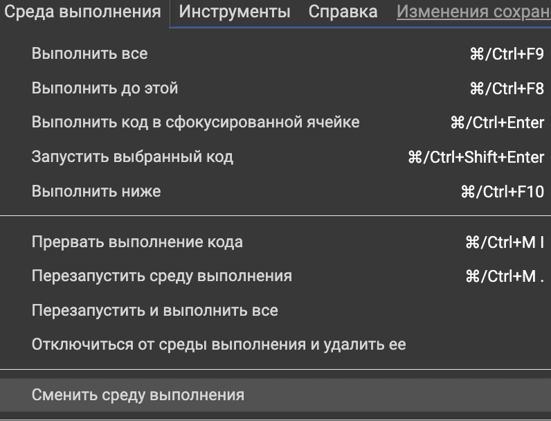
There is a chance that you only have a CPU out of the box. To fix this, select from the top menu
Runtime → Change runtime.
Setting the value
Hardware accelerator: GPU.
Installing dependencies.
!pip install diffusers transformers scipy ftfy "ipywidgets>=7,<8"Importing dependencies.
import os

import requests
import torch
import google.colab.output
from torch import autocast
from torch.nn import functional as F
from torchvision import transforms
from diffusers import (
    StableDiffusionPipeline, AutoencoderKL,
    UNet2DConditionModel, PNDMScheduler, LMSDiscreteScheduler
)
from diffusers.schedulers.scheduling_ddim import DDIMScheduler
from transformers import CLIPTextModel, CLIPTokenizer, CLIPProcessor, CLIPModel
from tqdm.auto import tqdm
from huggingface_hub import notebook_login
from PIL import Image, ImageDraw

device="cuda"

google.colab.output.enable_custom_widget_manager()
notebook_login()
And we see a celebos who asks for a token.

To get a token:
Login to the Hugging Face website https://huggingface.com/login
Accept model license https://huggingface.co/CompVis/stable-diffusion-v1-4
We generate a token https://huggingface.co/settings/tokens
Paste into Colab.

It’s time to write 3 lines of Python code – not a boy’s act, but a husband’s!
Download the network weights and load them into the video memory.
pipe = StableDiffusionPipeline.from_pretrained(
    'CompVis/stable-diffusion-v1-4',
    revision='fp16',
    tourch_dtype=torch.float16,
    use_auth_token=True
)
pipe = pipe.to(device)
Ask prompt and generate an image.
prompt="A grey sketch on paper of a Ferrari car, full car, pencil art"
with autocast(device):
    image = pipe(prompt)['images'][0]
image
We enjoy the result.
It is also possible to generate multiple images at once.
def image_grid(images, rows, cols):
    assert len(images) == rows * cols

    w, h = images[0].size
    grid = Image.new('RGB', size=(cols * w, rows * h))
    grid_w, grid_h = grid.size

    for i, img in enumerate(images):
        grid.paste(img, box=(i % cols * w, i // cols * h))
    return grid
nrows, ncols = 1, 3
prompts = [
'A grey sketch on paper of a Ferrari car, full car, pencil art'
] * nrows * ncols
with autocast(device):
images = pipe(prompts)['sample']
image_grid(images, rows=nrows, cols=ncols)We turn the drum. We get a super prize – a car in the amount of three pieces.

If you overdo it with the number of simultaneously generated images, then an error will occur.
RuntimeError: CUDA out of memory.If you look at the consumption of video memory using the command
!nvidia-smiWe will see that in my case (I tried nrows=2, ncols=3) 15 out of 16 Gb are occupied.

To deal with the error, you can restart the runtime from the top menu. In this case, the dependencies do not need to be reinstalled, they are cached for the duration of the session.
The main idea of the model
Let’s teach the neural network to draw pictures from nothing. And for inspiration, let’s look at physicists.
Remember what happens if you drop ink into water? The liquids will mix, the water will turn black. In physics, this process is called diffusion.
Stable Diffusion belongs to the class of diffusion models. The idea is to mix the image and Gaussian noise. And then train the neural network from noisy images to restore the originals.

If you apply pure noise to the input of such a neural network, then gradually it will turn it into a pretty picture. In Stable Diffusion, this is done by UNet.
The nuance is that a picture with a resolution of 512×512 consists of 262,144 pixels. If you apply the diffusion process to it directly, then the calculations will take a lot of time and memory, which complicates the process of training and inference. We want to generate images quickly and on relatively small video cards. Therefore, the images are mapped to a lower dimensional space (latent space), calculations are made there, and the result is decompressed back using the Variational Autoencoder (VAE).
It is not enough to generate a random picture from noise. We want to force the model to pay attention to the textual description that is given to it. For this, the Text Encoder from the CLIP model is used.
The Scheduler process controls the process – some algorithm that does not contain trainable parameters. It is responsible for how exactly we make noise in images.
Variational Autoencoder (VAE)
The Diffusers library uses the VAE implementation from Auto-Encoding Variational Bayes by Diederik P. Kingma and Max Welling.
The model consists of an encoder and a decoder.

The encoder takes as input a picture in the form of a tensor (1, 3, 512, 512), where 1 – batch size, 3 – RGB encoding. Returns a latent (compressed) representation – a dimension tensor (1, 4, 64, 64).
The decoder takes a tensor from the latent space as input and restores the original image with some accuracy. As a result, we have a network that can compress and decompress pictures.
Let’s load the model.
vae = AutoencoderKL.from_pretrained(
    'CompVis/stable-diffusion-v1-4', subfolder="vae", use_auth_token=True
)
vae = vae.to(device)
dict(vae.config)

> {
  'in_channels': 3,
  'out_channels': 3,
  'down_block_types': ['DownEncoderBlock2D',
    'DownEncoderBlock2D',
    'DownEncoderBlock2D',
    'DownEncoderBlock2D'],
  'up_block_types': ['UpDecoderBlock2D',
    'UpDecoderBlock2D',
    'UpDecoderBlock2D',
    'UpDecoderBlock2D'],
  'block_out_channels': [128, 256, 512, 512],
  'layers_per_block': 2,
  'act_fn': 'silu',
  'latent_channels': 4,
  'sample_size': 512,
  '_class_name': 'AutoencoderKL',
  '_diffusers_version': '0.3.0',
  '_name_or_path': 'CompVis/stable-diffusion-v1-4'
}
Let’s take a picture.
content = requests.get('https://i.ibb.co/qmcCRQJ/ferrari.png', stream=True).raw
car_img = Image.open(content)
car_img = car_img.resize((512, 512))
car_img
And we will display it in latent space using an encoder.
def preprocess(pil_image):
    pil_image = pil_image.convert("RGB")
    processing_pipe = transforms.Compose([
        transforms.Resize((512, 512)),
        transforms.ToTensor(),
        transforms.Normalize([0.5], [0.5]),
    ])
    tensor = processing_pipe(pil_image)
    tensor = tensor.reshape(1, 3, 512, 512)
    return tensor


def encode_vae(img):
    img_tensor = preprocess(img)
    with torch.no_grad():
        diag_gaussian_distrib_obj = vae.encode(img_tensor.to(device), return_dict=False)
        img_latent = diag_gaussian_distrib_obj[0].sample().detach().cpu()
        img_latent *= 0.18215
    return img_latent

car_latent = encode_vae(car_img)
car_latent.shape

> torch.Size([1, 4, 64, 64])
Got car_latent – a compressed representation of our picture with a dimension (1, 4, 64, 64).
Now let’s feed the image to the input of the decoder.
def decode_latents(latents):
    latents = 1 / 0.18215 * latents

    with torch.no_grad():
        images = vae.decode(latents)['sample']

    images = (images / 2 + 0.5).clamp(0, 1)
    images = images.detach().cpu().permute(0, 2, 3, 1).numpy()
    images = (images * 255).round().astype('uint8')
    pil_images = [Image.fromarray(image) for image in images]
    return pil_images

images = decode_latents(car_latent.to(device))
images[0]
We got something very similar to the input image. This allows models like Latent Diffusion to show good results using less computing resources due to operating in latent space.
CLIP
CLIP is a model from OpenAI that was trained on images and their descriptions from the Internet. The main beauty is that it displays pictures and texts in a single vector space. This allows you to measure the proximity between pictures and texts.

The model consists of a Text Encoder (Transformer) and an Image Encoder (ViT).
Let’s compare the picture that was submitted to the VAE input in the last section and the text descriptions:
clip_model = CLIPModel.from_pretrained("openai/clip-vit-base-patch32")
clip_processor = CLIPProcessor.from_pretrained("openai/clip-vit-base-patch32")

url="https://i.ibb.co/qmcCRQJ/ferrari.png"
image = Image.open(requests.get(url, stream=True).raw)

description_candidates = [
    'A grey sketch on paper of a Ferrari car, full car, pencil art',
    'a car',
    'a dinosaur',
]

inputs = clip_processor(text=description_candidates, images=image, return_tensors="pt", padding=True)
outputs = clip_model(**inputs)
logits_per_image = outputs.logits_per_image  # this is the image-text similarity score
probs = logits_per_image.softmax(dim=1)  # we can take the softmax to get the label probabilities

print(logits_per_image)
> [37.2948, 26.1819, 19.6026]

print(probs)
> [9.9999e-01, 1.4917e-05, 2.0718e-08]
We see that the description 'A grey sketch on paper of a Ferrari car, full car, pencil art' matches the picture with a probability of 0.9999, while the description 'a dinosaur' fits the same picture with a probability close to zero.
UNet
The workhorse under the hood is Stable Diffusion. It is this component that produces Denoising – iterative transformation of noise into the resulting image.

Previously, diffusion models were only able to restore images from noise, but did not take into account the textual description. Then they consisted of ResNet blocks – convolutional layers + skip connections.
In Stable Diffusion, everything is the same, but CrossAttention blocks are additionally used. They allow you to look in the CLIP Text Encoder so that the generated result matches the text description.
unet = UNet2DConditionModel.from_pretrained(
    'CompVis/stable-diffusion-v1-4', subfolder="unet", use_auth_token=True
)
unet = unet.to(device)
unet.config

> {
'sample_size': 64,
 'in_channels': 4,
 'out_channels': 4,
 'center_input_sample': False,
 'flip_sin_to_cos': True,
 'freq_shift': 0,
 'down_block_types': ['CrossAttnDownBlock2D',
  'CrossAttnDownBlock2D',
  'CrossAttnDownBlock2D',
  'DownBlock2D'],
 'up_block_types': ['UpBlock2D',
  'CrossAttnUpBlock2D',
  'CrossAttnUpBlock2D',
  'CrossAttnUpBlock2D'],
 'block_out_channels': [320, 640, 1280, 1280],
 'layers_per_block': 2,
 'downsample_padding': 1,
 'mid_block_scale_factor': 1,
 'act_fn': 'silu',
 'norm_num_groups': 32,
 'norm_eps': 1e-05,
 'cross_attention_dim': 768,
 'attention_head_dim': 8,
 '_class_name': 'UNet2DConditionModel',
 '_diffusers_version': '0.3.0',
 '_name_or_path': 'CompVis/stable-diffusion-v1-4'
}
At the end of the article, I will attach a link to Colab from the creators of Diffusers, where you can experiment with UNet and different Schedulers.
Putting together your pipeline
Let’s use the knowledge about VAE, CLIP, UNet and assemble a pipeline similar to the one we called through StableDiffusionPipeline in the second section of the article.
Let’s create a scheduler.
scheduler = LMSDiscreteScheduler(
    beta_start=0.00085,
    beta_end=0.012,
    beta_schedule="scaled_linear",
    num_train_timesteps=1000
)
Let’s write a function to get text embeddings for description'A grey sketch on paper of a Ferrari car, full car, pencil art'.
def get_text_embeds(prompt):
    text_input = tokenizer(
        prompt, padding='max_length', max_length=tokenizer.model_max_length,
        truncation=True, return_tensors="pt"
    )
    with torch.no_grad():
        text_embeddings = text_encoder(text_input.input_ids.to(device))[0]

    uncond_input = tokenizer(
        [''] * len(prompt), padding='max_length', max_length=tokenizer.model_max_length,
        truncation=True, return_tensors="pt"
    )
    with torch.no_grad():
        uncond_embeddings = text_encoder(uncond_input.input_ids.to(device))[0]

    text_embeddings = torch.cat([uncond_embeddings, text_embeddings])
    return text_embeddings


prompt="A grey sketch on paper of a Ferrari car, full car, pencil art"
test_embeds = get_text_embeds([prompt])
print(test_embeds)
print(test_embeds.shape)

> tensor([[[-0.3884,  0.0229, -0.0522,  ..., -0.4899, -0.3066,  0.0675],
         [-0.3711, -1.4497, -0.3401,  ...,  0.9489,  0.1867, -1.1034],
         [-0.5107, -1.4629, -0.2926,  ...,  1.0419,  0.0701, -1.0284],
         ...,
         [ 0.5668,  1.1076, -2.3770,  ..., -1.4189, -0.6171,  0.4183],
         [ 0.5545,  1.1131, -2.3889,  ..., -1.4055, -0.6261,  0.4250],
         [ 0.5227,  1.1315, -2.3088,  ..., -1.4146, -0.6122,  0.3927]]],
       device="cuda:0")

> torch.Size([2, 77, 768])
Let’s write a function that creates a random vector in latent space and performs Denoising using UNet and Scheduler, given test_embeds from the previous step.
def generate_latents(
    text_embeddings,
    height=512,
    width=512,
    num_inference_steps=50,
    guidance_scale=7.5,
    latents=None
):
    if latents is None:
        latents = torch.randn((
            text_embeddings.shape[0] // 2,
            unet.in_channels,
            height // 8,
            width // 8
        ))
    latents = latents.to(device)

    scheduler.set_timesteps(num_inference_steps)
    latents = latents * scheduler.sigmas[0]

    with autocast('cuda'):
        for i, t in tqdm(enumerate(scheduler.timesteps)):
            latent_model_input = torch.cat([latents] * 2)
            sigma = scheduler.sigmas[i]
            latent_model_input = latent_model_input / ((sigma ** 2 + 1) ** 0.5)

            with torch.no_grad():
                noise_pred = unet(latent_model_input, t, encoder_hidden_states=text_embeddings)['sample']

            noise_pred_uncond, noise_pred_text = noise_pred.chunk(2)
            noise_pred = noise_pred_uncond + guidance_scale * (noise_pred_text - noise_pred_uncond)

            latents = scheduler.step(noise_pred, i, latents)['prev_sample']
    return latents


test_latents = generate_latents(test_embeds)
print(test_latents)
print(test_latents.shape)

> tensor([[[[ 0.2196,  0.3412,  0.2564,  ...,  0.5965,  0.2621,  0.9491],
          [ 0.5094,  0.6396,  0.7730,  ...,  0.7261,  0.9269,  0.8177],
          [ 0.3972,  0.0753,  0.5931,  ...,  0.6357,  1.2942,  0.9378],
          ...,
          [ 0.0101,  0.1279, -0.3112,  ..., -0.5879, -0.3295, -0.4144],
          [-0.1014,  0.6407,  0.3716,  ..., -0.3444, -0.6487, -0.4429],
          [-0.1337, -0.0826, -0.1991,  ..., -0.4089, -0.5995, -0.4405]]]],
       device="cuda:0")

> torch.Size([1, 4, 64, 64])
Let’s feed the resulting tensor as input to the VAE decoder.
def decode_latents(latents):
latents = 1 / 0.18215 * latents
with torch.no_grad():
images = vae.decode(latents)['sample']
images = (images / 2 + 0.5).clamp(0, 1)
images = images.detach().cpu().permute(0, 2, 3, 1).numpy()
images = (images * 255).round().astype('uint8')
pil_images = [Image.fromarray(image) for image in images]
return pil_images
images = decode_latents(test_latents)
images[0]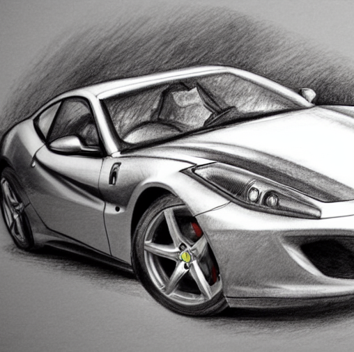 Telegramso you don’t miss new articles.