Regression Analysis Methods in Data Science

If we talk about mathematics in the context of Data Science, we can single out the three most frequently solved problems (although there are, of course, more problems):

Let’s talk about these tasks in more detail:

1. Regression Analysis Task or identifying dependencies (when we have a certain set of observations). In the graph above, you can see that there is a certain variable x and a certain variable y, and we observe the values ​​of y for a specific x. We know these points and know their coordinates, and we also know that x somehow affects y, that is, these two variables are dependent on each other. Naturally, we want to calculate the equation of their dependence – for this we use model classic paired linear regressionwhen it is assumed that their dependence can be described by a certain straight line. Accordingly, then the straight line coefficients are selected so as to minimize the error in the description of the data. And just on what kind of error (quality metric) will be selected, the actual result of constructing a linear regression depends.
2. Another task from data analysis is recommendation systems. This is when we say that there are, for example, online stores, they have a certain set of goods, and a person makes purchases. Based on this information, it is possible to provide a description of this person in vector space, and, having built this vector space, build a mathematical dependence of the probability with which this person will buy this or that product, knowing his previous purchases. Accordingly, we are talking about classification when we classify potential buyers according to the principles: “buy-not buy”, “interesting-uninteresting”, etc. There are various approaches: user-based and item-based.
3. The third area is computer vision. In the course of this task, we are trying to determine where the object of interest to us is located. This is actually a solution to the problem of minimizing errors by selecting specific pixels that form the image of the object.

In all three problems, there is optimization, error minimization, and the presence of one or another model that describes the dependence of variables. At the same time, inside each lies a representation of data that is decomposed into a vector description. In our article, we will pay special attention to the section that affects precisely regression models.

We already mentioned that there is a certain set of data pairs: X and Y. We know what values ​​Y takes with respect to X. If X is time, then we get a time series model in which Y is, say, the price of oil and at the same time, the ruble to dollar exchange rate, and X is a certain period of time from 2014 to 2018:

If you build graphically, it is clear that these two time series are interdependent. Having defined the concept of correlation, you can calculate the degree of their dependence, and then, if you know that some values ​​are perfectly correlated (the correlation is 1 or -1), you can use this either for forecasting tasks or for description tasks.

Consider the following illustration:

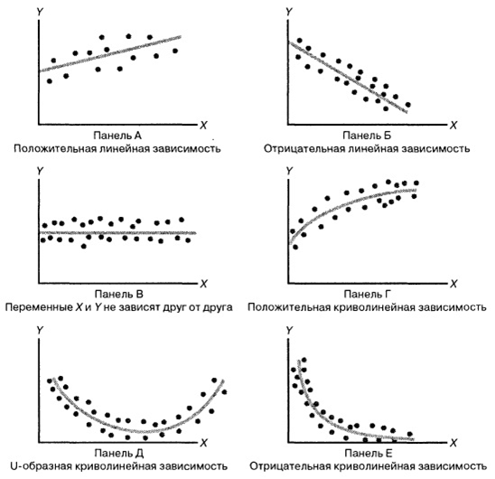
The most difficult part in creating a regression model is initially lay in her memory some specific function. For example, for Figure A it is Y = kX + b, for B it is Y = -kX + b, in figure C the “game” is equal to some number, the graph in figure D is most likely based on the root from “ X ”, at the base of D, possibly a parabola, and at the base of E – a hyperbole.

It turns out we choose some kind of data dependency model, and the types of dependence between random variables are different. Everything is not so obvious, because even in these simple drawings we see various dependencies. By choosing a specific relationship, we can use regression methods to calibrate the model.

The quality of your forecasts will depend on which model you choose. If we focus on linear regression models, then we assume that there is a certain set of real values:

The figure shows the 4 observed values ​​of X1, X2, X2, X4. For each of the X’s, the Y value is known (in our case, these are the points: P1, P2, P3, P4). These are the points that we actually observe on the data. Thus, we received a certain dataset. And for some reason, we decided that linear regression best describes the relationship between the X and the player. Then the whole question is how to construct the equation of a straight line Y = b₁ + b₂X where b₂ – slope coefficient, b₁ Is the intersection coefficient. The whole question is which b₂ and b₁ it is best to establish that this straight line describes the relationship between these variables as accurately as possible.

R points₁, R₂, R₃, R₄ – these are the values ​​that our model produces for the values ​​of X. What happens? Points P are points that we actually observe (actually collected), and points R are points that we observe in our model (those that it produces). What follows is insanely simple human logic: a model will be considered qualitative if and only if the points R are as close as possible to the points P.

If we construct the distance between these points for the same “X” (P₁ – R₁, P₂ – R₂ etc.), then we get what is called linear regression errors. We get deviations in linear regression, and these deviations are called U₁, U₂, U₃… U_n. And these errors can be either in plus or minus (we could overestimate or underestimate). To compare these deviations, they need to be analyzed. A very large and beautiful method is used here – squaring (squaring “kills” the sign). And the sum of the squares of all the deviations in mathematical statistics is called RSS (Residual Sum of Squares). By minimizing RSS by b₁ and minimizing RSS by b₂, we get the optimal coefficients that are actually derived least squares method.

After we built the regression, we determined the optimal coefficients b₁ and b₂, and we have a regression equation, the problems do not end there, and the problem continues to develop. The fact is that if the regression itself is marked on one graph, all the values ​​that we have, as well as the average values ​​of the “games”, then the sum of the squared errors can be clarified.

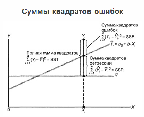
At the same time, it is considered useful to display regression prediction errors with respect to variable X. See the figure below:

We got some kind of regression and drew the real data that is. We got the distance from each real value to the regression. And we drew it with respect to the zero value for the corresponding values ​​of X. And in the figure above we see a really very bad picture: errors depend on X. Some correlation dependence is explicitly expressed: the farther along the X we move, the greater the significance of errors. This is very bad. The presence of correlation in this case indicates that we mistakenly took the regression model, and there was some parameter that we “did not think of” or simply overlooked. After all, if all the variables are placed inside the model, the errors should be completely random and should not depend on what your factors are equal. Errors must be with the same probability distributionotherwise your predictions will be erroneous. If you have drawn the errors of your model on the plane and met a diverging triangle, it is better to start all from scratch and completely recount the model.

By analyzing errors, you can even immediately understand where they miscalculated, what type of error they made. And here we can not fail to mention the Gauss-Markov theorem:

The theorem determines the conditions under which the estimates obtained by the least squares method are the best, consistent, effective in the class of linear unbiased estimates.

The conclusion can be drawn as follows: now we understand that the area of ​​constructing a regression model is, in a sense, the culmination of mathematics, because it merges all possible sections at once, which may be useful in data analysis, for example:

• linear algebra with data representation methods;
• mathematical analysis with optimization theory and means of analysis of functions;
• probability theory with means of describing random events and quantities and modeling the relationship between variables.

Colleagues, I suggest all the same, not limited to reading and see the whole webinar. The article did not include moments related to linear programming, optimization in regression models, and other details that may be useful to you.