Monte Carlo Blackjack Strategy Optimization

Reinforced training took the world of Artificial Intelligence. Starting from AlphaGo and AlphaStar, an increasing number of activities that were previously dominated by humans are now conquered by AI agents based on reinforcement training. In short, these achievements depend on optimizing the actions of the agent in a particular environment to achieve maximum reward. In the last few articles from GradientCrescent, we have looked at various fundamental aspects of reinforced learning, from the basics of bandit systems and policy-based approaches to optimizing reward-based behavior in Markov environments. All these approaches required complete knowledge of our environment. Dynamic programming, for example, requires that we have a complete probability distribution of all possible state transitions. However, in reality, we find that most systems cannot be fully interpreted, and that probability distributions cannot be obtained explicitly due to complexity, inherent uncertainty, or limitations in computational capabilities. As an analogy, we consider the meteorologist's task – the number of factors involved in weather forecasting can be so great that it is impossible to accurately calculate the probability.

For such cases, training methods such as Monte Carlo are the solution. The term Monte Carlo is commonly used to describe any random sampling approach. In other words, we do not predict knowledge about our environment, but learn from experience by going through exemplary sequences of states, actions and rewards obtained as a result of interaction with the environment. These methods work by directly observing the rewards returned by the model during normal operation in order to judge the average value of its states. Interestingly, even without any knowledge of the dynamics of the environment (which should be considered as the probability distribution of state transitions), we can still get optimal behavior to maximize rewards.

As an example, consider the result of a roll of 12 dice. Considering these throws as a single state, we can average these results in order to get closer to the true predicted result. The larger the sample, the more accurately we will come closer to the actual expected result.

The average expected amount on 12 dice for 60 shots is 41.57

This kind of sampling-based assessment may seem familiar to the reader, since such sampling is also performed for k-bandit systems. Instead of comparing different bandits, Monte Carlo methods are used to compare different policies in Markov environments, determining the value of the state as a certain policy is followed until the work is completed.

Monte Carlo estimation of the state value

In the context of reinforcement learning, Monte Carlo methods are a way to evaluate the significance of the state of a model by averaging sample results. Due to the need for a terminal state, Monte Carlo methods are inherently applicable to episodic environments. Because of this limitation, Monte Carlo methods are usually considered “autonomous”, in which all updates are performed after reaching the terminal state. A simple analogy with finding a way out of a maze can be given – an autonomous approach would force the agent to reach the very end before using the intermediate experience gained to try to reduce the time it takes to go through the maze. On the other hand, with the online approach, the agent will constantly change its behavior already during the passage of the maze, maybe he will notice that the green corridors lead to dead ends and decide to avoid them, for example. We will discuss online approaches in one of the following articles.

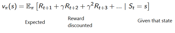
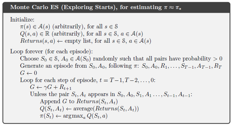
The Monte Carlo method can be formulated as follows:

To better understand how the Monte Carlo method works, consider the state transition diagram below. The reward for each state transition is displayed in black, a discount factor of 0.5 is applied to it. Let's leave aside the actual value of the state and focus on calculating the results of one throw.

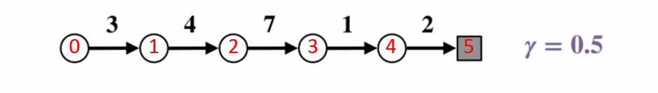
State transition diagram. The status number is shown in red, the result is black.

Given that the terminal state returns a result equal to 0, let's calculate the result of each state, starting with the terminal state (G5). Please note that we have set the discount factor to 0.5, which will result in a weighting towards later states.

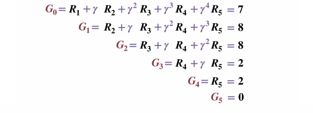
Or more generally:

To avoid storing all the results in a list, we can perform the update of the state value in the Monte Carlo method gradually, using an equation that has some similarities with the traditional gradient descent:

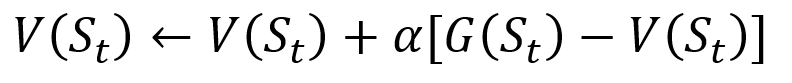
Monte Carlo incremental update procedure. S is the state, V is its value, G is its result, and A is the step value parameter.

As part of reinforcement training, Monte Carlo methods can even be classified as First-visit or Every visit. In short, the difference between the two is how many times a state can be visited a passage before the Monte Carlo update. The Monte Carlo First-visit method estimates the value of all states as the average value of the results after single visits to each state before the work is completed, while the Monte Carlo Every visit method averages the results after n visits until the work is completed. We will use the Monte Carlo First-visit throughout this article because of its relative simplicity.

Monte Carlo Policy Management

If the model cannot provide the policy, Monte Carlo can be used to evaluate state-action values. This is more useful than just the meaning of the states, since the idea of ​​the meaning of each action (q) in this state allows the agent to automatically generate a policy from observations in an unfamiliar environment.

More formally, we can use Monte Carlo to evaluate q (s, a, pi)expected result when starting from state s, action a, and subsequent policy Pi. Monte Carlo methods remain the same, except that there is an additional dimension of actions taken for a certain state. State-action pair (s, a)is visited over the passage if the state is ever visited s and it takes action a. Similarly, the evaluation of value-actions can be carried out using the approaches “First-visit” and “Every visit”.

As in dynamic programming, we can use a generalized iteration policy (GPI) to form a policy from observing state-action values.

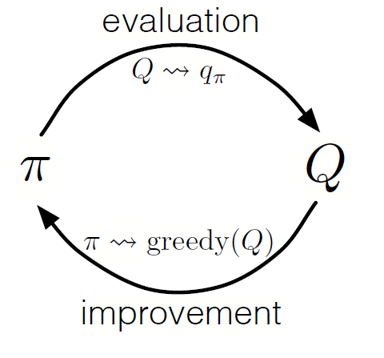
By alternating the steps of policy evaluation and policy improvement, and including research to ensure that all possible actions are visited, we can achieve the optimal policy for each condition. For the Monte Carlo GPI, this rotation is usually done after the end of each pass.

Monte Carlo GPI

Blackjack strategy

To better understand how the Monte Carlo method works in practice in the task of assessing various state values, let's take a step-by-step demonstration of the blackjack game. To begin, let's determine the rules and conditions of our game:

• We will play only against the dealer, there will be no other players. This will allow us to consider the hands of the dealer as part of the environment.
• The value of cards with numbers equal to the nominal values. The value of the picture cards: Jack, King and Queen is 10. The value of the ace can be 1 or 11 depending on the choice of the player.
• Both sides receive two cards. Two cards of the player lie face up, one of the dealer’s cards also lies face up.
• The goal of the game is that the amount of cards in hand is <= 21. A value greater than 21 is a bust, if both sides have a value of 21, then the game is played in a draw.
• After the player has seen his cards and the first dealer’s card, the player can choose to take him a new card (“yet”) or not (“enough”) until he is satisfied with the sum of the card values ​​in his hand.
• Then the dealer shows his second card – if the resulting amount is less than 17, he is obliged to take cards until he reaches 17 points, after which he does not take the card anymore.

Let's see how the Monte Carlo method works with these rules.

Round 1.

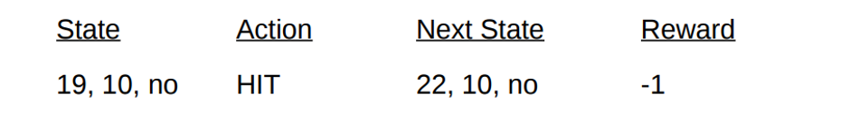
You gain a total of 19. But you try to catch luck by the tail, take a chance, get 3 and go broke. When you went broke, the dealer had only one open card with a sum of 10. This can be represented as follows:

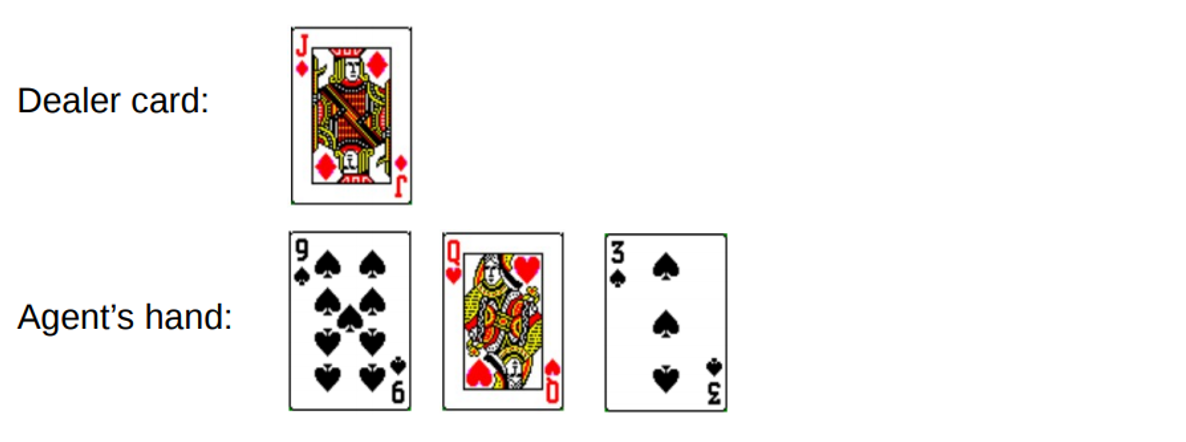
If we go broke, our reward for the round is -1. Let's set this value as the result of the penultimate state, using the following format [Сумма агента, Сумма дилера, туз?]:

Well, now we're out of luck. Let's move on to another round.

Round 2.

You type a total of 19. This time you decide to stop. The dealer dials 13, takes a card and goes broke. The penultimate state can be described as follows.

Let's describe the conditions and rewards that we received in this round:

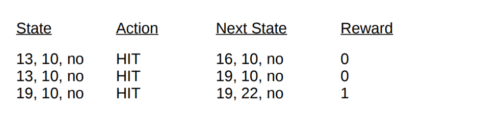
With the end of the passage, we can now update the values ​​of all our states in this round using the calculated results. Taking a discount factor of 1, we simply distribute our new reward by hand, as was done with state transitions earlier. Since the condition V (19, 10, no) previously returned -1, we calculate the expected return value and assign it to our state:

Final state values ​​for demonstration using blackjack as an example.

Implementation

Let's write a blackjack game using the first-visit Monte Carlo method to find out all the possible state values ​​(or various combinations on hand) in the game using Python. Our approach will be based on the approach of Sudharsan et. al .. As usual, you can find all the code from the article on our GitHub.

To simplify the implementation, we will use gym from OpenAI. Think of the environment as an interface for starting a blackjack game with a minimal amount of code, this will allow us to focus on implementing reinforced learning. Conveniently, all collected information about conditions, actions and rewards is stored in variables "Observation"that accumulate during current game sessions.

Let's start by importing all the libraries we need to get and collect our results.

import gym
import numpy as np
from matplotlib import pyplot
import matplotlib.pyplot as plt
from mpl_toolkits.mplot3d import Axes3D
from collections import defaultdict
from functools import partial
% matplotlib inline
plt.style.use (‘ggplot’)

Next let's initialize our environment gym and define a policy that will coordinate the actions of our agent. In fact, we will continue to take the card until the amount in our hand reaches 19 or more, after which we will stop.

#Observation here encompassess all data about state that we need, as well as reactions to it
env = gym.make (‘Blackjack-v0’)
#Define a policy where we hit until we reach 19.
# actions here are 0-stand, 1-hit
def sample_policy (observation):
  score, dealer_score, usable_ace = observation
  return 0 if score> = 19 else 1

Let's define a method for generating pass data using our policy. We will store information about the status, actions taken and remuneration for the action.

def generate_episode (policy, env):
# we initialize the list for storing states, actions, and rewards
  states, actions, rewards = [], [], []
# Initialize the gym environment
  observation = env.reset ()
  while True:
# append the states to the states list
    states.append (observation)
# now, we select an action using our sample_policy function and append the action to actions list
    action = sample_policy (observation)
    actions.append (action)
# We perform the action in the environment according to our sample_policy, move to the next state
    observation, reward, done, info = env.step (action)
    rewards.append (reward)
# Break if the state is a terminal state (i.e. done)
    if done:
      break
  return states, actions, rewards

Finally, let's define the Monte Carlo prediction function first visit. First, we initialize an empty dictionary to store the current state values ​​and a dictionary that stores the number of records for each state in different passes.

def first_visit_mc_prediction (policy, env, n_episodes):
# First, we initialize the empty value table as a dictionary for storing the values ​​of each state
  value_table = defaultdict (float)
  N = defaultdict (int)

For each pass, we call our method generate_episodeto receive information about the values ​​of the conditions and rewards received after the onset of the state. We also initialize the variable to store our incremental results. Then we get the reward and the current state value for each state visited during the pass, and increase our variable returns by the value of the reward per step.

for _ in range (n_episodes):
# Next, we generate the epsiode and store the states and rewards
  states, _, rewards = generate_episode (policy, env)
  returns = 0
# Then for each step, we store the rewards to a variable R and states to S, and we calculate
  for t in range (len (states) - 1, -1, -1):
    R = rewards
    S = states
    returns + = R
# Now to perform first visit MC, we check if the episode is visited for the first time, if yes,
#This is the standard Monte Carlo Incremental equation.
# NewEstimate = OldEstimate + StepSize (Target-OldEstimate)
    if S not in states[:t]:
      N[S] + = 1
      value_table[S] + = (returns - value_table[S]) / N[S]
return value_table

Let me remind you that since we are implementing the first-visit of Monte Carlo, we visit one state in one pass. Therefore, we do a conditional check on the state dictionary to see if the state has been visited. If this condition is met, we are able to calculate the new value using the previously defined procedure for updating the state values ​​using the Monte Carlo method and increase the number of observations for this state by 1. Then we repeat the process for the next pass in order to ultimately obtain the average value of the result .

Let's run what we have and look at the results!

value = first_visit_mc_prediction (sample_policy, env, n_episodes = 500000)
for i in range (10):
  print (value.popitem ())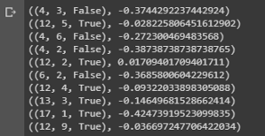

Conclusion of a sample showing the state values ​​of various combinations on the hands in blackjack.

We can continue to make Monte Carlo observations for 5000 passes and build a distribution of state values ​​that describes the values ​​of any combination in the hands of the player and dealer.

def plot_blackjack (V, ax1, ax2):
  player_sum = np.arange (12, 21 + 1)
  dealer_show = np.arange (1, 10 + 1)
  usable_ace = np.array ([False, True])
  state_values ​​= np.zeros ((len (player_sum), len (dealer_show), len (usable_ace)))
  for i, player in enumerate (player_sum):
    for j, dealer in enumerate (dealer_show):
      for k, ace in enumerate (usable_ace):
        state_values[i, j, k] = V[player, dealer, ace]
  X, Y = np.meshgrid (player_sum, dealer_show)
  ax1.plot_wireframe (X, Y, state_values[:, :, 0])
  ax2.plot_wireframe (X, Y, state_values[:, :, 1])
  for ax in ax1, ax2: ax.set_zlim (-1, 1)
    ax.set_ylabel (‘player sum’)
    ax.set_xlabel (‘dealer sum’)
    ax.set_zlabel (‘state-value’)
fig, axes = pyplot.subplots (nrows = 2, figsize = (5, 8), subplot_kw = {'projection': '3d'})
axes[0].set_title ('state-value distribution w / o usable ace')
axes[1].set_title ('state-value distribution w / usable ace')
plot_blackjack (value, axes[0]axes[1])

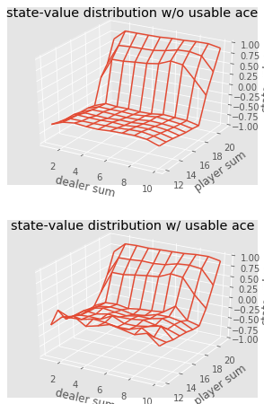
Visualization of the status values ​​of various combinations in blackjack.

So, let's summarize what we learned.

• Sampling-based learning methods allow us to evaluate state and action-state values ​​without any transition dynamics, simply by sampling.
• Monte Carlo approaches are based on random sampling of the model, observing the rewards returned by the model, and collecting information during normal operation to determine the average value of its states.
• Using Monte Carlo methods, a generalized iteration policy is possible.
• The value of all possible combinations in the hands of the player and dealer in blackjack can be estimated using multiple Monte Carlo simulations, opening the way for optimized strategies.

This concludes the introduction to the Monte Carlo method. In our next article, we will move on to teaching methods of the form Temporal Difference learning.

Sources:

Sutton et. al, Reinforcement Learning
White et. al, Fundamentals of Reinforcement Learning, University of Alberta
Silva et. al, Reinforcement Learning, UCL
Platt et. Al, Northeaster University

That's all. See you on the course!