Fundamentals of Generative Adversarial Networks

What are GANs and what can they do?

At a high level, GANs are neural networks that learn to generate realistic samples of the data they were trained on. For example, given photographs of handwritten digits, GANs learn how to create realistic photographs of more handwritten digits. More impressively, GANs can even learn how to create realistic photographs of people, such as the one below.

So how do GANs work? Essentially, GANs study the distribution of an object of interest. For example. GANs trained on handwritten digits learn the distribution of data. Once the distribution of the data is learned, the GAN can simply choose from the distribution to create realistic images.

Data distribution

To reinforce our understanding of data distribution, let’s look at the following example. Let’s say we have the following 6 images below.

Each image is a grayish rectangle, and for simplicity, let’s assume that each image consists of only 1 pixel. In other words, there is only one grayish pixel in each image.

Now suppose each pixel has a possible value between -1 and 1, where the white pixel has a value of -1 and the black pixel has a value of 1. So 6 gray images would have the following pixel values:

What do we know about the distribution of pixel values? Well, just by checking, we know that most pixel values ​​are around 0, with a few values ​​approaching extreme values ​​(-1 and 1). Therefore, we can assume that the distribution is Gaussian with a mean of 0.

Note. Given more samples, getting a Gaussian distribution of this data is trivial by calculating the mean and standard deviation. However, this is not our goal, since it is difficult to calculate the distribution of data over complex objects, unlike this simple example.

This data distribution is useful because it allows us to generate more grayscale images like the 6 above. To create more similar images, we can randomly select from a distribution.

While calculating the underlying distribution of gray pixels can be trivial, calculating the distribution of cats, dogs, cars, or any other complex object often turns out to be mathematically intractable.

How then do we learn the underlying distribution of complex objects? The obvious answer is to use neural networks. With enough data, we can train a neural network to learn any complex feature, such as the underlying distribution of the data.

Generator – Distribution Learning Model

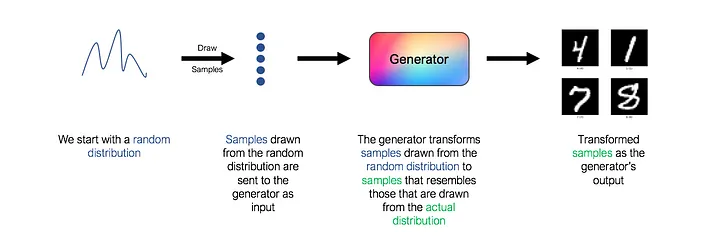
In GAN, a generator is a neural network that learns the underlying distribution of data. To be more specific, the generator takes as input a random distribution (also known as “noise” in the GAN literature) and learns a mapping function that maps the input to the desired output, which is the actual underlying distribution of the data.

However, note that the architecture above is missing a key component. What loss function should we use to train the generator? How do we know if the generated images really resemble real handwritten numbers? As always, the answer use a neural network “. This second network is known as the discriminator.

Discriminator – opponent of the Generator

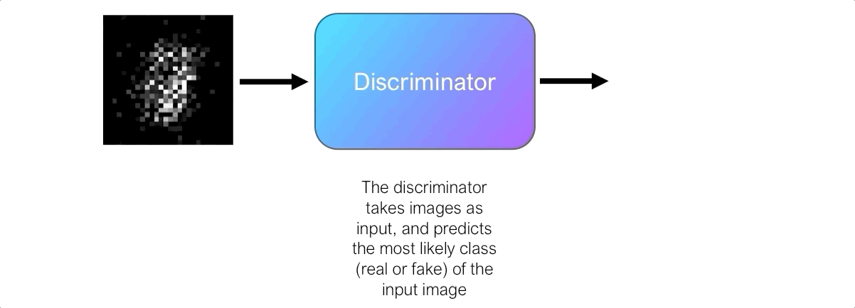
The role of the discriminator is to evaluate the quality of the output images of the generator. Technically, the discriminator is a binary classifier. It takes images as input and outputs the probability that the image is real (i.e. the actual training image) or fake (i.e. received from a generator).

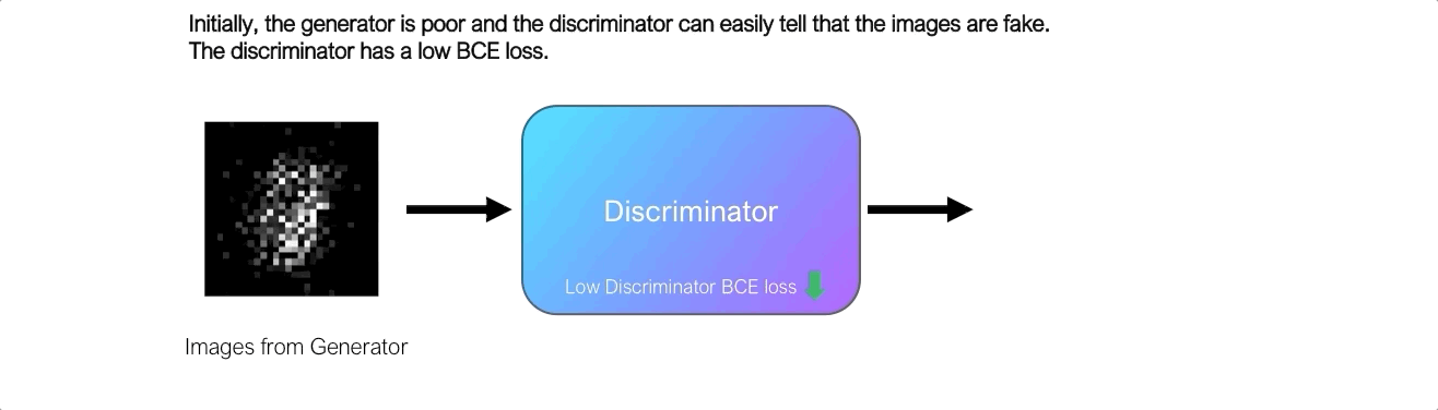
At first, the generator struggles to create images that look real, and the discriminator can easily distinguish real images from fake ones without making too many mistakes. Since the discriminator is a binary classifier, we can quantify the performance of the discriminator using the binary cross entropy loss.

The loss of the discriminator is an important signal for the generator. We recall earlier that the generator itself does not know whether the generated images are similar to real ones. However, the generator can use the BCE loss of the discriminator as a signal to get feedback on the images it generates.

Here’s how it works. We send the images generated by the generator to the discriminator, and it predicts the probability that the image is real. Initially, when the generator is bad, the discriminator can easily classify the images as fake, resulting in low BCE loss. However, over time, the generator improves and the discriminator starts making more errors, misclassifying fake images as real ones, resulting in higher BCE loss. Therefore, the loss of the BCE of the discriminator signals the quality of the image output by the generator, and the generator seeks to maximize this loss.

The generator uses the discriminator loss as a measure of the quality of the images it generates. The task of the generator is to adjust its weights in such a way that the BCE loss from the discriminator is maximized, effectively “fooling” the discriminator.

Discriminator Training

But what about the discriminator? So far, we have assumed that we have a perfectly working discriminator from the very beginning. However, this assumption is incorrect and the discriminator also requires training.

Since the discriminator is a binary classifier, its training procedure is simple. We will provide the discriminator with a set of labeled real and fake images and use the BCE loss to tune the discriminator weights. We train the discriminator to recognize real and fake images, preventing the generator from “cheating” the discriminator.

GAN – a story about two networks

Let’s now put everything together and see how GANs work.

By now, you know that GANs are made up of two interconnected networks, a generator and a discriminator. In conventional GANs, generators and discriminators are simple feed-forward neural networks.

What is unique to GANs is that the generator and discriminator are trained in turn, hostile to each other.

To train the generator, we use as input a noise vector selected from a random distribution. In practice, we use a vector of length 100 taken from a Gaussian distribution as the noise vector. The input goes through a series of fully connected layers in a feedforward neural network. The output of the generator is an image, which in our MNIST example is 28x28array. The generator feeds its output to the discriminator and uses the discriminator’s BCE loss to adjust its weights to maximize the discriminator’s loss.

To train the discriminator, we use labeled images from the generator as well as real images as input. The discriminator learns to classify images as real or fake and is trained with the BCE loss function.

In practice, we train the generator and discriminator in turn, one after the other. This learning scheme is similar to a two-player minimax adversarial game, as the generator seeks to maximize losses discriminator, and the discriminator seeks minimize their own losses.

Building your own GAN

Now that we understand the theory behind GANs, let’s put it into practice by building our own GAN from scratch with PyTorch!

First of all, let’s add the MNIST dataset. Library torchvisionallows us to easily retrieve the MNIST dataset. We will do some standard image normalization before flattening. 28x28MNIST images to 784tensor. This alignment is necessary because the layers in the network are fully connected layers.

import torch
import torch.nn as nn
from torch.utils.data import DataLoader
from torchvision import transforms, datasets

mnist_transforms = transforms.Compose([transforms.ToTensor(),
                                       transforms.Normalize(mean=0.5, std=0.5),
                                       transforms.Lambda(lambda x: x.view(-1, 784))])

data = datasets.MNIST(root="/data/MNIST", download=True, transform=mnist_transforms)

mnist_dataloader = DataLoader(data, batch_size=128, shuffle=True, num_workers=4) 

Next, let’s write the code for the generator class. From what we saw earlier, a generator is just a feedforward neural network that takes 100length tensor and outputs 784tensor. In the generator, the size of dense layers is usually doubled after each layer (256, 512, 1024).

class Generator(nn.Module):
  '''
  Generator class. Accepts a tensor of size 100 as input as outputs another
  tensor of size 784. Objective is to generate an output tensor that is
  indistinguishable from the real MNIST digits 
  '''
  
  def __init__(self):
    super().__init__()
    self.layer1 = nn.Sequential(nn.Linear(in_features=100, out_features=256),
                                nn.LeakyReLU())
    self.layer2 = nn.Sequential(nn.Linear(in_features=256, out_features=512),
                                nn.LeakyReLU())
    self.layer3 = nn.Sequential(nn.Linear(in_features=512, out_features=1024),
                                nn.LeakyReLU())
    self.output = nn.Sequential(nn.Linear(in_features=1024, out_features=28*28),
                                nn.Tanh())

  def forward(self, x):
    x = self.layer1(x)
    x = self.layer2(x)
    x = self.layer3(x)
    x = self.output(x)
    return x

It was easy, wasn’t it? Now let’s write the code for the discriminator class. The discriminator is also a feedforward neural network that accepts 784length tensor and produces a size tensor 1, denoting the probability that the input belongs to class 1 (real image). Unlike the generator, we halve the size of the dense layers after each layer (1024, 512, 256).

class Discriminator(nn.Module):
  '''
  Discriminator class. Accepts a tensor of size 784 as input and outputs
  a tensor of size 1 as  the predicted class probabilities
  (generated or real data)
  '''

  def __init__(self):
    super().__init__()
    self.layer1 = nn.Sequential(nn.Linear(in_features=28*28, out_features=1024),
                                nn.LeakyReLU())
    self.layer2 = nn.Sequential(nn.Linear(in_features=1024, out_features=512),
                                nn.LeakyReLU())
    self.layer3 = nn.Sequential(nn.Linear(in_features=512, out_features=256),
                                nn.LeakyReLU())
    self.output = nn.Sequential(nn.Linear(in_features=256, out_features=1),
                                nn.Sigmoid())
    
  def forward(self, x):
    x = self.layer1(x)
    x = self.layer2(x)
    x = self.layer3(x)
    x = self.output(x)
    return x

Now we are going to create a GAN class which includes both a generator class and a discriminator class. This GAN class will contain code to train the generator and discriminator in turn, following the learning pattern we discussed earlier. We are going to use for this PyTorch Lightning to simplify our code and cut down on boilerplate.

import pytorch_lightning as pl

class GAN(pl.LightningModule):

  def __init__(self):
    super().__init__()
    self.generator = Generator()
    self.discriminator = Discriminator()
    # After each epoch, we generate 100 images using the noise
    # vector here (self.test_noises). We save the output images
    # in a list (self.test_progression) for plotting later.
    self.test_noises = torch.randn(100,1,100, device=device)
    self.test_progression = []

  def forward(self, z):
    """
    Generates an image using the generator
    given input noise z
    """
    return self.generator(z)

  def generator_step(self, x):
    """
    Training step for generator
    1. Sample random noise
    2. Pass noise to generator to
       generate images
    3. Classify generated images using
       the discriminator
    4. Backprop loss to the generator
    """
    
    # Sample noise
    z = torch.randn(x.shape[0], 1, 100, device=device)

    # Generate images
    generated_imgs = self(z)

    # Classify generated images
    # using the discriminator
    d_output = torch.squeeze(self.discriminator(generated_imgs))

    # Backprop loss. We want to maximize the discriminator's
    # loss, which is equivalent to minimizing the loss with the true
    # labels flipped (i.e. y_true=1 for fake images). We do this
    # as PyTorch can only minimize a function instead of maximizing
    g_loss = nn.BCELoss()(d_output,
                           torch.ones(x.shape[0], device=device))

    return g_loss

  def discriminator_step(self, x):
    """
    Training step for discriminator
    1. Get actual images
    2. Predict probabilities of actual images and get BCE loss
    3. Get fake images from generator
    4. Predict probabilities of fake images and get BCE loss
    5. Combine loss from both and backprop loss to discriminator
    """
    
    # Real images
    d_output = torch.squeeze(self.discriminator(x))
    loss_real = nn.BCELoss()(d_output,
                             torch.ones(x.shape[0], device=device))

    # Fake images
    z = torch.randn(x.shape[0], 1, 100, device=device)
    generated_imgs = self(z)
    d_output = torch.squeeze(self.discriminator(generated_imgs))
    loss_fake = nn.BCELoss()(d_output,
                             torch.zeros(x.shape[0], device=device))

    return loss_real + loss_fake

  def training_step(self, batch, batch_idx, optimizer_idx):
    X, _ = batch

    # train generator
    if optimizer_idx == 0:
      loss = self.generator_step(X)
    
    # train discriminator
    if optimizer_idx == 1:
      loss = self.discriminator_step(X)

    return loss

  def configure_optimizers(self):
    g_optimizer = torch.optim.Adam(self.generator.parameters(), lr=0.0002)
    d_optimizer = torch.optim.Adam(self.discriminator.parameters(), lr=0.0002)
    return [g_optimizer, d_optimizer], []

  def training_epoch_end(self, training_step_outputs):
    epoch_test_images = self(self.test_noises)
    self.test_progression.append(epoch_test_images)

Now we can train our GAN. We will train it with the GPU for 100 epochs.

device = torch.device("cuda:0" if torch.cuda.is_available() else "cpu")

model = GAN()

trainer = pl.Trainer(max_epochs=100, gpus=1)
trainer.fit(model, mnist_dataloader)

Visualization of generated images

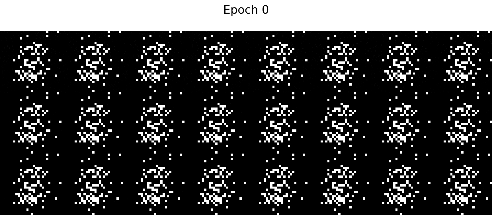
It remains only to visualize the generated images. IN training_epoch_end()function from our GAN class above, we saved the images output by the generator after each training epoch to a list.

We can visualize these images by plotting them on a grid. The code below randomly selects 10 images generated after the 100th training epoch and plots them on the grid.

import numpy as np
from matplotlib import pyplot as plt, gridspec

# Convert images from torch tensor to numpy array
images = [i.detach().cpu().numpy() for i in model.test_progression]

epoch_to_plot = 100
nrow = 3
ncol = 8

# randomly select 10 images for plotting
indexes = np.random.choice(range(100), nrow*ncol, replace=False)

fig = plt.figure(figsize=((ncol+1)*2, (nrow+1)*2)) 
fig.suptitle('Epoch {}'.format(epoch_to_plot), fontsize=30)

gs = gridspec.GridSpec(nrow, ncol,
         wspace=0.0, hspace=0.0, 
         top=1.-0.5/(nrow+1), bottom=0.5/(nrow+1), 
         left=0.5/(ncol+1), right=1-0.5/(ncol+1)) 

for i in range(nrow):
    for j in range(ncol):
        idx = i*ncol + j
        img = np.reshape(images[epoch_to_plot-1][indexes[idx]], (28,28))
        ax = plt.subplot(gs[i,j])
        ax.imshow(img, cmap='gray')
        ax.axis('off')

Finally, as promised, we will create the animation shown at the top of the post. Using FuncAnimationfunction in matplotlibwe will animate the images on the chart frame by frame.

import numpy as np
from matplotlib import pyplot as plt, gridspec, rc
from matplotlib.animation import FuncAnimation
rc('animation', html="jshtml")

images = [i.detach().cpu().numpy() for i in model.test_progression]

nrow = 3
ncol = 8

indexes = np.random.choice(range(100), nrow*ncol, replace=False)

fig = plt.figure(figsize=((ncol+1)*2, (nrow+1)*2)) 

gs = gridspec.GridSpec(nrow, ncol,
         wspace=0.0, hspace=0.0, 
         top=1.-0.5/(nrow+1), bottom=0.5/(nrow+1), 
         left=0.5/(ncol+1), right=1-0.5/(ncol+1)) 

for i in range(nrow):
  for j in range(ncol):
    ax = plt.subplot(gs[i,j])
    ax.axis('off')

def animate(frame):
  fig.suptitle('Epoch {}'.format(frame), fontsize=30)
  ret = []
  for i in range(nrow):
    for j in range(ncol):
      idx = i*ncol + j
      img = np.reshape(images[frame][indexes[idx]], (28,28))
      ax = fig.axes[idx]
      ax.imshow(img, cmap='gray')
      ret.append(ax.get_images()[0])
  return ret
    
anim = FuncAnimation(fig, animate, frames=100, interval=50, blit=True)

What’s next?

Congratulations! You have reached the end of this lesson. I hope you enjoyed reading this as much as I enjoyed writing it.