Computer vision lessons in Python + OpenCV from the very beginning. Part 7
In the last lesson, we learned some ways to find regions of interest in an image. Let me remind you what we did:
-
tried to find by color (most often you don’t need to do this);
-
tried to find a round sign using the HoughCircles function (sometimes it works);
-
and we also studied morphological operations (opening-closing).
Today’s tutorial will be more in-depth about working with paths, as often the path helps to highlight features in images, as well as areas of interest (thanks to the path, we can capture the shape of the object).
First, let’s remember how to find contours:
import cv2
import numpy as np

my_photo = cv2.imread('DSCN1311.JPG')
filterd_image  = cv2.medianBlur(my_photo,7)
img_grey = cv2.cvtColor(filterd_image,cv2.COLOR_BGR2GRAY)

#set a thresh
thresh = 100

#get threshold image
ret,thresh_img = cv2.threshold(img_grey, thresh, 255, cv2.THRESH_BINARY)

#find contours
contours, hierarchy = cv2.findContours(thresh_img, cv2.RETR_TREE, cv2.CHAIN_APPROX_SIMPLE)

#create an empty image for contours
img_contours = np.uint8(np.zeros((my_photo.shape[0],my_photo.shape[1])))

cv2.drawContours(img_contours, contours, -1, (255,255,255), 1)

cv2.imshow('origin', my_photo) # выводим итоговое изображение в окно
cv2.imshow('res', img_contours) # выводим итоговое изображение в окно

cv2.waitKey()
cv2.destroyAllWindows()
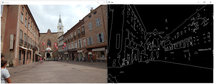
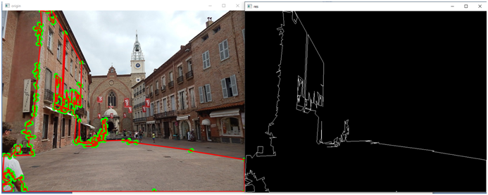
Please note that before selecting the contours, we use filtering. Here’s what we got:
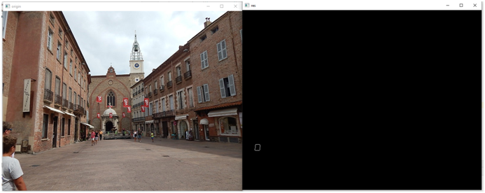
Without filtering, we would get this (for comparison, on the right without a filter, on the left with a filter):

Now let’s see what exactly findContours returns and how to work with it:
contours, hierarchy = cv2.findContours(thresh_img, cv2.RETR_TREE, cv2.CHAIN_APPROX_SIMPLE)
print(type(contours),type(hierarchy))
We got the output:
Thus, the contour itself is an ordinary tuple, and the second returned value is a numpy array. If we look at this tuple with a debugger, we can see that the elements of this tuple are a numpy array:

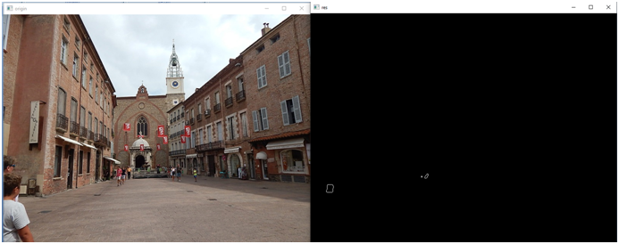
In other words, the function returns a whole set of contours. In theory, you can work with each of the contours separately. Let’s, for example, display the fourth (it will actually be at number 3, we count from scratch) contour:
img_contours = np.uint8(np.zeros((my_photo.shape[3],my_photo.shape[1])))Here is what we will see in the picture:
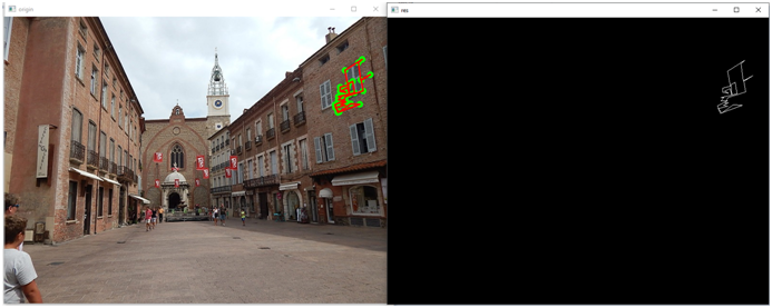
You can display several contours at once:
sel_countours=[]
sel_countours.append(contours[3])
sel_countours.append(contours[7])
sel_countours.append(contours[8])
cv2.drawContours(img_contours, sel_countours, -1, (255,255,255), 1)
Here’s what we’ll see:
Let’s find the largest contour:
max=0
sel_countour=None
for countour in contours:
    if countour.shape[0]>max:
        sel_countour=countour
        max=countour.shape[0]

cv2.drawContours(img_contours, [sel_countour], -1, (255,255,255), 1)
We look:

I must say that the contour can be stored both as points and as segments, depending on the approximation parameter set:
contours, hierarchy = cv2.findContours(thresh_img, cv2.RETR_TREE, cv2.CHAIN_APPROX_SIMPLE)In our case, Simple is set, which means that the contour is stored in the form of segments, if we draw by points, then the contour will not work:
for point in sel_countour:
    y=int(point[0][1])
    x=int(point[0][0])
    img_contours[y,x]=255
We look:

But if you tell the findContours function to search for contours without approximation:
contours, hierarchy = cv2.findContours(thresh_img, cv2.RETR_TREE, cv2.CHAIN_APPROX_NONE)Then the contour will be as in the previous picture.
On the other hand, if you have approximation turned on, then you can draw a contour by connecting the points with lines:
last_point=None
for point in sel_countour:
    curr_point=point[0]
    if not(last_point is None):
        x1=int(last_point[0])
        y1=int(last_point[1])
        x2=int(curr_point[0])
        y2=int(curr_point[1])
        cv2.line(img_contours, (x1, y1), (x2, y2), 255, thickness=1)
    last_point=curr_point
It will be the same as in the first picture.
And so, the findContours function returns grouped sets of points, which are the points of the contour (or the ends of the contour segments, depending on the type of approximation).
We can further approximate the resulting contour:
import cv2
import numpy as np
import os
img = cv2.imread("DSCN1311.JPG")
gray = cv2.cvtColor(img, cv2.COLOR_BGR2GRAY)
thresh = 100

#get threshold image
ret,thresh_img = cv2.threshold(gray, thresh, 255, cv2.THRESH_BINARY)

# find contours without approx
contours,_ = cv2.findContours(thresh_img,cv2.RETR_TREE,cv2.CHAIN_APPROX_NONE)

max=0
sel_countour=None
for countour in contours:
    if countour.shape[0]>max:
        sel_countour=countour
        max=countour.shape[0]

# calc arclentgh
arclen = cv2.arcLength(sel_countour, True)

# do approx
eps = 0.0005
epsilon = arclen * eps
approx = cv2.approxPolyDP(sel_countour, epsilon, True)

# draw the result
canvas = img.copy()
for pt in approx:
    cv2.circle(canvas, (pt[0][0], pt[0][1]), 7, (0,255,0), -1)

cv2.drawContours(canvas, [approx], -1, (0,0,255), 2, cv2.LINE_AA)

img_contours = np.uint8(np.zeros((img.shape[0],img.shape[1])))
cv2.drawContours(img_contours, [approx], -1, (255,255,255), 1)


cv2.imshow('origin', canvas) # выводим итоговое изображение в окно
cv2.imshow('res', img_contours) # выводим итоговое изображение в окно

cv2.waitKey()
cv2.destroyAllWindows()
Let’s see what happens:
We can control the accuracy of the approximation by changing the value of the eps variable. Let’s put, for example, instead of 0.0005 the value 0.005 and the picture will be completely different:

And now let’s take a closer look at the piece of code responsible for the approximation:
# calc arclentgh
arclen = cv2.arcLength(sel_countour, True)

# do approx
eps = 0.0005
epsilon = arclen * eps
approx = cv2.approxPolyDP(sel_countour, epsilon, True)
The arcLength function returns the arc length of a path. Let’s try to see the lengths of different contours. But let’s first sort the contours in decreasing order of their lengths. To do this, we define a custom sorting function:
def custom_sort(countour):
    return -countour.shape[0]
Now we can sort the contours:
contours=list(contours)
contours.sort(key=custom_sort)
The longest path will be first:
sel_countour=contours[0]

# calc arclentgh
arclen = cv2.arcLength(sel_countour, True)
print(arclen)
The rest of the contours will be smaller, for example, here is the contour at index 5:
Move on. Having obtained the length of the contour arc, we calculate the so-called epsilon, a parameter that characterizes the accuracy of the approximation. The criterion is the maximum distance between the original curve and its approximation.
The approximate contour is, in fact, the same points connected by segments, so it can be derived like this:
last_point=None
for point in approx:
    curr_point=point[0]
    if not(last_point is None):
        x1=int(last_point[0])
        y1=int(last_point[1])
        x2=int(curr_point[0])
        y2=int(curr_point[1])
        cv2.line(img_contours, (x1, y1), (x2, y2), 255, thickness=1)
    last_point=curr_point
And so, now we know what the resulting contour is – these are segments. We can even approximate these segments, getting a rougher contour, thereby getting rid of small details. But what to do next? As I already wrote in part 4, the contour can be turned into a graph or into geometric primitives, thereby describing it invariantly to displacement, rotation, and even scaling.
Now we will try to create such an invariant description of the object. Let it be an ordinary ballpoint pen:

It is logical to assume that you need to work with the longest contour. Let’s find him, we already know how:
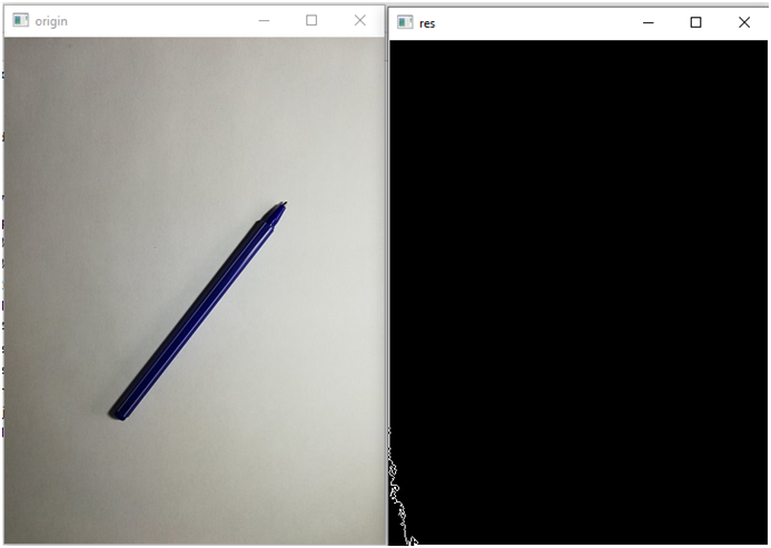
No, you didn’t guess, you’ll have to sort it out. Fortunately, the contour turned out to be the second longest:
contours,_ = cv2.findContours(thresh_img,cv2.RETR_TREE,cv2.CHAIN_APPROX_NONE)
contours=list(contours)
contours.sort(key=custom_sort)
sel_countour=contours[1]
We approximate it:

As it turned out, with a value of eps=0.005, the contour has only 7 elements:
eps = 0.005
epsilon = arclen * eps
approx = cv2.approxPolyDP(sel_countour, epsilon, True)
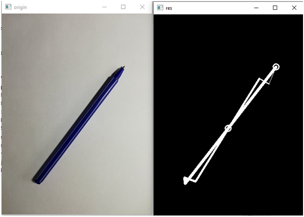
print(len(approx))Let’s see how the contour will be selected in other positions:


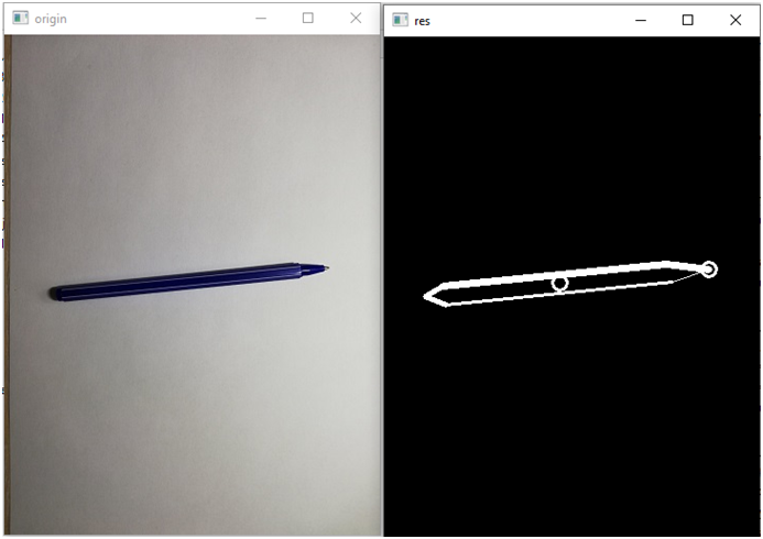
In the latter case, we got, by the way, not 7, but 9 elements. In short, there is an ambush with a shadow. In general, it is necessary to somehow get rid of small details. But how? Raise the approximation threshold? Let’s make 0.01:

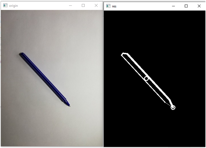
The number of elements became 6. In other photographs, by the way, it is also 6. Such a hexagon:

Now let’s try to describe this contour invariantly. You can do this in two ways:
– angles between contour faces;
– the ratio of the lengths of the sides.
Both methods will be invariant to translation, rotation and scaling. But the question is: which side to count? One option is to find the center of the contour and take the point farthest from it as the beginning. How to find a center? As the average coordinate of all contour points.
sum_x=0.0
sum_y=0.0
for point in approx:
    x = float(point[0][0])
    y = float(point[0][1])
    sum_x+=x
    sum_y+=y
xc=sum_x/float(len((approx)))
yc=sum_y/float(len((approx)))
Let’s display the center after the contour is drawn:
cv2.circle(img_contours, (int(xc), int(yc)), 7, (255,255,255), 2)
Find the point furthest from the center:
max=0
beg_point=-1
for i in range(0,len(approx)):
    point=approx[i]
    x = float(point[0][0])
    y = float(point[0][1])
    dx=x-xc
    dy=y-yc
    r=math.sqrt(dx*dx+dy*dy)
    if r>max:
        max=r
        beg_point=i
Let’s draw it:
point=approx[beg_point]
x = float(point[0][0])
y = float(point[0][1])
cv2.circle(img_contours, (int(x), int(y)), 7, (255,255,255), 2)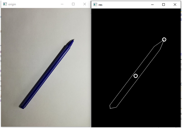
Now we just go around the contour clockwise, starting from the found point. To do this, we convert the coordinates of the points to polar ones and sort them by angle.
We calculate polar coordinates with the following function:
def get_polar_coordinates(x0,y0,x,y,xc,yc):
    #Первая координата в полярных координатах - радиус
    dx=xc-x
    dy=yc-y
    r=math.sqrt(dx*dx+dy*dy)

    #Вторая координата в полярных координатах - узел, вычислим относительно начальной точки
    dx0=xc-x0
    dy0=yc-y0
    r0 = math.sqrt(dx0 * dx0 + dy0 * dy0)
    scal_mul=dx0*dx+dy0*dy
    cos_angle=scal_mul/r/r0
    sgn=dx0*dy-dx*dy0 #опредедляем, в какую сторону повернут вектор
    angle=math.acos(cos_angle)
    if sgn<0:
        angle=2*math.pi-angle
    return angle,r
Here we set the start point of the report, the desired point and our center. The first coordinate is the radius, we will calculate it using the Pythagorean theorem. We find the angle through the scalar product. Here, however, there is an ambush. Through the dot product, we will calculate the angle between the vectors, but not the direction. To calculate it, we need to find define matrices of vectors. This sign will be the direction of rotation. But we need not just a negative angle, otherwise, when sorting, the first point will not be the beginning of the report, but the point with the most negative angle. Therefore, if the direction is in the other direction, then subtract this angle from the angle of 2 pi radians (360 degrees).
If it is not clear, then I will now clearly demonstrate the problem. But, let’s sort first:
polar_coordinates=[]
x0=approx[beg_point][0][0]
y0=approx[beg_point][0][1]
print(x0,y0)
for point in approx:
    x = int(point[0][0])
    y = int(point[0][1])
    angle,r=get_polar_coordinates(x0,y0,x,y,xc,yc)
    polar_coordinates.append(((angle,r),(x,y)))
print(polar_coordinates)
polar_coordinates.sort(key=polar_sort)
And then we draw:
img_contours = np.uint8(np.zeros((img.shape[0],img.shape[1])))
size=len(polar_coordinates)
for i in range(1,size):
    _ , point1=polar_coordinates[i-1]
    _, point2 = polar_coordinates[i]
    x1,y1=point1
    x2,y2=point2
    cv2.line(img_contours, (x1, y1), (x2, y2), 255, thickness=i)
_ , point1=polar_coordinates[size-1]
_, point2 = polar_coordinates[0]
x1,y1=point1
x2,y2=point2
cv2.line(img_contours, (x1, y1), (x2, y2), 255, thickness=size)
Let’s see what happened:

In order to see the bypass, I made the first lines thin, but as they go around, they become thicker.
And now let’s remove our manipulations with determining the direction of rotation from the function of converting to polar coordinates:
def get_polar_coordinates(x0,y0,x,y,xc,yc):
    #Первая координата в полярных координатах - радиус
    dx=xc-x
    dy=yc-y
    r=math.sqrt(dx*dx+dy*dy)

    #Вторая координата в полярных координатах - узел, вычислим относительно начальной точки
    dx0=xc-x0
    dy0=yc-y0
    r0 = math.sqrt(dx0 * dx0 + dy0 * dy0)
    scal_mul=dx0*dx+dy0*dy
    cos_angle=scal_mul/r/r0
    #sgn=dx0*dy-dx*dy0 #опредедляем, в какую сторону повернут вектор
    angle=math.acos(cos_angle)
    #if sgn<0:
    #    angle=2*math.pi-angle
    return angle,r
And then what nonsense will turn out:
So, let’s put back what we commented out and continue.
Let’s proceed to the invariant description. The angles between the edges of the contour. Here we will assume that the angles are positive and less than 180 degrees, that is, we will not do those manipulations with determining the direction. Although … it’s even better to define not the angles, but the cosines of the angles, they will take values from 0 to 1. In fact, this will already be a regular vector that we can input to some classification algorithm, for example, a neural network.
And so, the function for calculating the cosine of the angle between the faces (!!!!!!!):
def get_cos_edges(edges):
    dx1, dy1, dx2, dy2=edges
    r1 = math.sqrt(dx1 * dx1 + dy1 * dy1)
    r2 = math.sqrt(dx2 * dx2 + dy2 * dy2)
    return (dx1*dx2+dy1*dy2)/r1/r2
Please note that we are specifying relative coordinates in the function, not absolute ones. And we need to calculate them, for this we will write another function:
def get_coords(item1, item2, item3):
    _, point1 = item1
    _, point2 = item2
    _, point3 = item3
    x1, y1 = point1
    x2, y2 = point2
    x3, y3 = point3
    dx1=x1-x2
    dy1=y1-y2
    dx2=x3-x2
    dy2=y3-y2
    return dx1,dy1,dx2,dy2
Well, actually, the code for obtaining an invariant description:
coses=[]
coses.append(get_cos_edges(get_coords(polar_coordinates[size-1],polar_coordinates[0],polar_coordinates[1])))
for i in range(1,size-1):
    coses.append(get_cos_edges(get_coords(polar_coordinates[i-1], polar_coordinates[i],polar_coordinates[i+1])))
coses.append(get_cos_edges(get_coords(polar_coordinates[size-2], polar_coordinates[size-1],polar_coordinates[0])))

print(coses)
Let’s run the program and see these vectors for different handle positions:

Generated vector:
[0.8435094506704439, -0.9679482843035412, -0.7475204740128089, 0.12575426475263257, -0.7530074822433576, -0.9513518107379842]
Let’s look in another position:
Generated vector:
[0.8997284651496198, -0.9738348113021638, -0.886281044605172, 0.6119832801209469, -0.9073303511520623, -0.9760783176138438]
As you can see, the first two digits turned out to be close, the third a little further, the fourth has changed a lot, the penultimate one as well, but the last one also almost coincided.
For the purity of the experiment, in one more position:
Vector:
[0.8447017514267182, -0.968529494204698, -0.20124730714807806, -0.4685934718394871, -0.7702667523702886, -0.9517100095171195]
We see a similar situation.
Of course, it is not good that some numbers of the vector “float” strongly (again, the shadow interferes, be it amiss). This will complicate identification. But we still have another option, which we will look at in the next lesson. And now, in conclusion, the lesson, I will give the entire code of the example:
import cv2
import numpy as np
import math
import os
img = cv2.imread("Samples/1.jpg")
gray = cv2.cvtColor(img, cv2.COLOR_BGR2GRAY)
thresh = 100

def custom_sort(countour):
    return -countour.shape[0]

def polar_sort(item):
    return item[0][0]

def get_cos_edges(edges):
    dx1, dy1, dx2, dy2=edges
    r1 = math.sqrt(dx1 * dx1 + dy1 * dy1)
    r2 = math.sqrt(dx2 * dx2 + dy2 * dy2)
    return (dx1*dx2+dy1*dy2)/r1/r2

def get_polar_coordinates(x0,y0,x,y,xc,yc):
    #Первая координата в полярных координатах - радиус
    dx=xc-x
    dy=yc-y
    r=math.sqrt(dx*dx+dy*dy)

    #Вторая координата в полярных координатах - узел, вычислим относительно начальной точки
    dx0=xc-x0
    dy0=yc-y0
    r0 = math.sqrt(dx0 * dx0 + dy0 * dy0)
    scal_mul=dx0*dx+dy0*dy
    cos_angle=scal_mul/r/r0
    sgn=dx0*dy-dx*dy0 #опредедляем, в какую сторону повернут вектор
    if cos_angle>1:
        if cos_angle>1.0001:
            raise Exception("Что-то пошло не так")
        cos_angle=1
    angle=math.acos(cos_angle)
    if sgn<0:
        angle=2*math.pi-angle
    return angle,r

def get_coords(item1, item2, item3):
    _, point1 = item1
    _, point2 = item2
    _, point3 = item3
    x1, y1 = point1
    x2, y2 = point2
    x3, y3 = point3
    dx1=x1-x2
    dy1=y1-y2
    dx2=x3-x2
    dy2=y3-y2
    return dx1,dy1,dx2,dy2

#get threshold image
ret,thresh_img = cv2.threshold(gray, thresh, 255, cv2.THRESH_BINARY)

# find contours without approx
contours,_ = cv2.findContours(thresh_img,cv2.RETR_TREE,cv2.CHAIN_APPROX_NONE)
contours=list(contours)
contours.sort(key=custom_sort)
sel_countour=contours[1]

# calc arclentgh
arclen = cv2.arcLength(sel_countour, True)

# do approx
eps = 0.01
epsilon = arclen * eps
approx = cv2.approxPolyDP(sel_countour, epsilon, True)

sum_x=0.0
sum_y=0.0
for point in approx:
    x = float(point[0][0])
    y = float(point[0][1])
    sum_x+=x
    sum_y+=y
xc=sum_x/float(len((approx)))
yc=sum_y/float(len((approx)))

max=0
beg_point=-1
for i in range(0,len(approx)):
    point=approx[i]
    x = float(point[0][0])
    y = float(point[0][1])
    dx=x-xc
    dy=y-yc
    r=math.sqrt(dx*dx+dy*dy)
    if r>max:
        max=r
        beg_point=i

polar_coordinates=[]
x0=approx[beg_point][0][0]
y0=approx[beg_point][0][1]

for point in approx:
    x = int(point[0][0])
    y = int(point[0][1])
    angle,r=get_polar_coordinates(x0,y0,x,y,xc,yc)
    polar_coordinates.append(((angle,r),(x,y)))

polar_coordinates.sort(key=polar_sort)

img_contours = np.uint8(np.zeros((img.shape[0],img.shape[1])))
size=len(polar_coordinates)
for i in range(1,size):
    _ , point1=polar_coordinates[i-1]
    _, point2 = polar_coordinates[i]
    x1,y1=point1
    x2,y2=point2
    cv2.line(img_contours, (x1, y1), (x2, y2), 255, thickness=i)
_ , point1=polar_coordinates[size-1]
_, point2 = polar_coordinates[0]
x1,y1=point1
x2,y2=point2
cv2.line(img_contours, (x1, y1), (x2, y2), 255, thickness=size)

cv2.circle(img_contours, (int(xc), int(yc)), 7, (255,255,255), 2)

coses=[]
coses.append(get_cos_edges(get_coords(polar_coordinates[size-1],polar_coordinates[0],polar_coordinates[1])))
for i in range(1,size-1):
    coses.append(get_cos_edges(get_coords(polar_coordinates[i-1], polar_coordinates[i],polar_coordinates[i+1])))
coses.append(get_cos_edges(get_coords(polar_coordinates[size-2], polar_coordinates[size-1],polar_coordinates[0])))

print(coses)

point=approx[beg_point]
x = float(point[0][0])
y = float(point[0][1])
cv2.circle(img_contours, (int(x), int(y)), 7, (255,255,255), 2)

cv2.imshow('origin', img) # выводим итоговое изображение в окно
cv2.imshow('res', img_contours) # выводим итоговое изображение в окно

cv2.waitKey()
cv2.destroyAllWindows()