Calculation and analysis of the correlation ratio using Python

Formulation of the problem

In the statistical analysis of dependencies between quantitative variables, situations arise when it is of interest to calculate and analyze such an indicator as correlation ratio (η).

This indicator is undeservedly overlooked in most mathematical packages available to users.

In this analysis, we will consider methods for calculating and analyzing η means Python.

Let’s not go into theory η written in sufficient detail, for example, in [1, с.73], [2, с.412], [3, с.609]), but remember the main properties η:

η characterizes the degree of tightness any correlation (both linear and non-linear), in contrast to the Pearson correlation coefficient rwhich characterizes tightness only linear connections. Condition r=0 means the absence of a linear correlation between the quantities, but at the same time, a non-linear correlation can exist between them (η>0).
η takes values from 0 to 1; at η=0 there is no correlation η=1 the connection is considered functional; the degree of closeness of communication can be assessed using various generally accepted scales, for example, according to the Chaddock scale, etc.
Value η² characterizes the proportion of variation explained by the correlation between the considered variables.
η cannot be less than the absolute value r: η ≥ |r|.
η asymmetrical with respect to the variables under study, i.e. η_XY ≠ η_YX.
For calculation η it is necessary to have empirical data of the experiment with repetitions; if we have just two sets of variable values X and Y, then the data must be grouped. This conclusion is, in general, obvious – if an attempt is made to calculate η for ungrouped data, we get the result η=1.

Grouping data for calculation η consists in splitting the range of values of variables X and Y into intervals, counting the frequencies of data falling into intervals and forming correlation table.

Important note: features of the method for calculating the correlation ratio, especially when the form of the relationship is close to linear, and η close to unity can lead to results that are generally absurd, for example:

when the condition η ≥ |r| is violated;
when r will be significant, η No;
when the lower limit of the confidence interval for η will be less than 0 or the upper bound will be greater than 1.

This must be taken into account when performing the analysis.

So, let’s move on to the calculations.

Formation of initial data

As initial data, consider the dependence of the flow rate average monthly vehicle fuel consumption (l/100 km) (FuelFlow) from average monthly mileage (km) (Mileage).

Load the source data from the csv file (the source data is available in my GitHub repository):

fuel_df = pd.read_csv(
    filepath_or_buffer="data/fuel_df.csv",
    sep=';',
    index_col="Number")
dataset_df = fuel_df.copy()    # создаем копию исходной таблицы для работы
display(dataset_df.head())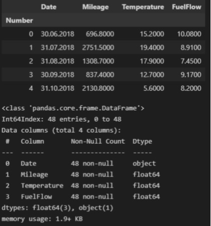

Downloaded DataFrame contains the following columns:

month – month (in Excel format)
Mileage – monthly mileage (km)
temperature – average monthly temperature (°C)
fuel flow – average monthly fuel consumption (l/100 km)

Save the variables we need Mileage and fuel flow as numpy.ndarray.

X = np.array(dataset_df['Mileage'])
Y = np.array(dataset_df['FuelFlow'])

For the convenience of further work, let’s create a separate DataFrame from two variables – X and Y:

data_XY_df = pd.DataFrame({
    'X': X,
    'Y': Y})

Setting up report titles (for further generation of charts):

# Общий заголовок проекта
Task_Project = "Расчет и анализ корреляционного отношения средствами Python"
# Заголовок, фиксирующий момент времени
AsOfTheDate = ""
# Заголовок раздела проекта
Task_Theme = "Анализ расхода топлива автомобиля"
# Общий заголовок проекта для графиков
Title_String = f"{Task_Project}\n{AsOfTheDate}"
# Наименования переменных
Variable_Name_X = "Среднемесячный пробег (км)"
Variable_Name_Y = "Среднемесячный расход топлива автомобиля (л/100 км)"

Visualization and primary data processing

Let us preliminarily weed out anomalous values (outliers). We will not dwell on this procedure in detail; it is not the purpose of this analysis.

mask1 = data_XY_df['X'] > 200
mask2 = data_XY_df['X'] < 2000
data_XY_df = data_XY_df[mask1 & mask2]

X = np.array(data_XY_df['X'])
Y = np.array(data_XY_df['Y'])

Descriptive statistics of the original data:

data_XY_df.describe()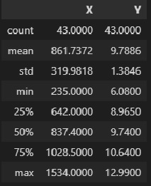

Let’s visualize the initial data:

fig, axes = plt.subplots(figsize=(297/INCH, 210/INCH))
fig.suptitle(Task_Theme)
axes.set_title('Зависимость расхода топлива от пробега')
data_df = data_XY_df
sns.scatterplot(
    data=data_df,
    x='X', y='Y',
    label="эмпирические данные",
    s=50,
    ax=axes)
axes.set_xlabel(Variable_Name_X)
axes.set_ylabel(Variable_Name_Y)
#axes.tick_params(axis="x", labelsize=f_size+4)
#axes.tick_params(axis="y", labelsize=f_size+4)
#axes.legend(prop={'size': f_size+6})
plt.show()
fig.savefig('graph/scatterplot_XY_sns.png', orientation = "portrait", dpi = 300)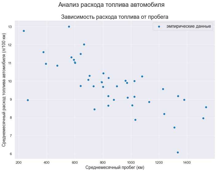

For a visual assessment of sample data, we will build histograms and box plots:

fig = plt.figure(figsize=(420/INCH, 297/INCH))
ax1 = plt.subplot(2,2,1)
ax2 = plt.subplot(2,2,2)
ax3 = plt.subplot(2,2,3)
ax4 = plt.subplot(2,2,4)
fig.suptitle(Task_Theme)
ax1.set_title('X')
ax2.set_title('Y')

# инициализация данных
data_df = data_XY_df
X_mean = data_df['X'].mean()
X_std = data_df['X'].std(ddof = 1)
Y_mean = data_df['Y'].mean()
Y_std = data_df['Y'].std(ddof = 1)
bins_hist="sturges"    # выбор числа интервалов ('auto', 'fd', 'doane', 'scott', 'stone', 'rice', 'sturges', 'sqrt')

# данные для графика плотности распределения X
xmin = np.amin(data_df['X'])
xmax = np.amax(data_df['X'])
nx = 100
hx = (xmax - xmin)/(nx - 1)
x1 = np.linspace(xmin, xmax, nx)
xnorm1 = sps.norm.pdf(x1, X_mean, X_std)
kx = len(np.histogram(X, bins=bins_hist, density=False)[0])
xnorm2 = xnorm1*len(X)*(xmax-xmin)/kx

# данные для графика плотности распределения Y
ymin = np.amin(Y)
ymax = np.amax(Y)
ny = 100
hy = (ymax - ymin)/(ny - 1)
y1 = np.linspace(ymin, ymax, ny)
ynorm1 = sps.norm.pdf(y1, Y_mean, Y_std)
ky = len(np.histogram(Y, bins=bins_hist, density=False)[0])
ynorm2 = ynorm1*len(Y)*(ymax-ymin)/ky

# гистограмма распределения X
ax1.hist(
    data_df['X'],
    bins=bins_hist,
    density=False,
    histtype="bar",    # 'bar', 'barstacked', 'step', 'stepfilled'
    orientation='vertical',   # 'vertical', 'horizontal'
    color = "#1f77b4",
    label="эмпирическая частота")
ax1.plot(
    x1, xnorm2,
    linestyle = "-",
    color = "r",
    linewidth = 2,
    label="теоретическая нормальная кривая")
ax1.axvline(X_mean, color="magenta", label="среднее значение")
ax1.axvline(np.median(data_df['X']), color="orange", label="медиана")
ax1.legend(fontsize = f_size+4)

# гистограмма распределения Y
ax2.hist(
    data_df['Y'],
    bins=bins_hist,
    density=False,
    histtype="bar",    # 'bar', 'barstacked', 'step', 'stepfilled'
    orientation='vertical',   # 'vertical', 'horizontal'
    color = "#1f77b4",
    label="эмпирическая частота")    
ax2.plot(
    y1, ynorm2,
    linestyle = "-",
    color = "r",
    linewidth = 2,
    label="теоретическая нормальная кривая")
ax2.axvline(Y_mean, color="magenta", label="среднее значение")
ax2.axvline(np.median(data_df['Y']), color="orange", label="медиана")
ax2.legend(fontsize = f_size+4)

# коробчатая диаграмма X
sns.boxplot(
    #data=corn_yield_df,
    x=data_df['X'],
    orient="h",
    width=0.3,
    ax=ax3)

# коробчатая диаграмма Y
sns.boxplot(
    #data=corn_yield_df, 
    x=data_df['Y'], 
    orient="h", 
    width=0.3, 
    ax=ax4)

# подписи осей 
ax3.set_xlabel(Variable_Name_X)
ax4.set_xlabel(Variable_Name_Y)

plt.show()
fig.savefig('graph/scatterplot_boxplot_X_Y_sns.png', orientation = "portrait", dpi = 300)

Before proceeding to further calculations, we check the initial data for compliance with the normal distribution law.

It is necessary to perform such a check, since only for normally distributed data can we subsequently use generally accepted statistical analysis procedures: checking the significance of a correlation relationship, constructing confidence intervals, etc.

To check the normality of the distribution, we use the Shapiro-Wilk test:

# функция для обработки реализации теста Шапиро-Уилка
def Shapiro_Wilk_test(data):
    data = np.array(data)
    result = sci.stats.shapiro(data)
    s_calc = result.statistic    # расчетное значение статистики критерия
    a_calc = result.pvalue    # расчетный уровень значимости
    
    print(f"Расчетный уровень значимости: a_calc = {round(a_calc, DecPlace)}")
    print(f"Заданный уровень значимости: a_level = {round(a_level, DecPlace)}")
    
    if a_calc >= a_level:
        conclusion_ShW_test = f"Так как a_calc = {round(a_calc, DecPlace)} >= a_level = {round(a_level, DecPlace)}" + \
            ", то гипотеза о нормальности распределения по критерию Шапиро-Уилка ПРИНИМАЕТСЯ"
    else:
        conclusion_ShW_test = f"Так как a_calc = {round(a_calc, DecPlace)} < a_level = {round(a_level, DecPlace)}" + \
            ", то гипотеза о нормальности распределения по критерию Шапиро-Уилка ОТВЕРГАЕТСЯ"
    print(conclusion_ShW_test)

# проверка нормальности распределения переменной X
Shapiro_Wilk_test(X)

# проверка нормальности распределения переменной Y
Shapiro_Wilk_test(Y)

So, the hypothesis of the normal distribution of the initial data is accepted, which allows us to further use statistical tools for interval estimation of the quantity ηtesting hypotheses, etc.

We proceed to the actual calculation of the correlation relationship.

Calculation and analysis of the correlation relationship

1. Let’s group the initial data according to both features X and Y:

Let’s create a new variable matrix_XY_df to work with grouped data:

matrix_XY_df = data_XY_df.copy()

Determine the number of grouping intervals (use the Sturgess formula); the minimum number of intervals must be at least 2:

# объем выборки для переменных X и Y
n_X = len(X)
n_Y = len(Y)

# число интервалов группировки
group_int_number = lambda n: round (3.31*log(n_X, 10)+1) if round (3.31*log(n_X, 10)+1) >=2 else 2

K_X = group_int_number(n_X)
K_Y = group_int_number(n_Y)
print(f"Число интервалов группировки для переменной X: {K_X}")
print(f"Число интервалов группировки для переменной Y: {K_Y}")

Let’s group the data using the library tools pandasfor this we use the function pandas.cut. As a result, we obtain new features cut_X and cut_Xwhich show which of the intervals a particular value falls into X and Y. Add the received new features to the DataFrame matrix_XY_df:

cut_X = pd.cut(X, bins=K_X)
cut_Y = pd.cut(Y, bins=K_Y)

matrix_XY_df['cut_X'] = cut_X
matrix_XY_df['cut_Y'] = cut_Y

display(matrix_XY_df.head())

Now we can get the correlation table using the function pandas.crosstab:

CorrTable_df = pd.crosstab(
    index=matrix_XY_df['cut_X'],
    columns=matrix_XY_df['cut_Y'],
    rownames=['cut_X'],
    colnames=['cut_Y'])

display(CorrTable_df)

# проверка правильности подсчета частот по интервалам
print(f"sum = {np.sum(np.array(CorrTable_df))}")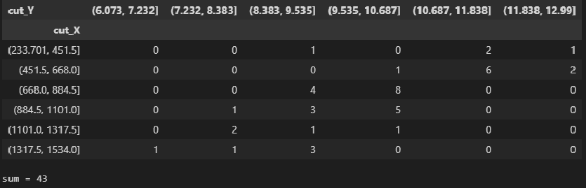

Function pandas.crosstab also allows you to create more even and more readable boundaries of grouping intervals by setting them manually. For calculation η this is not of fundamental importance, but in some cases it can be useful.

For example, let’s manually set the boundaries of the grouping intervals for X and Y:

bins_X = pd.IntervalIndex.from_tuples([(200, 400), (400, 600), (600, 800), (800, 1000), (1000, 1200), (1200, 1400), (1400, 1600)])
cut_X = pd.cut(X, bins=bins_X)

bins_Y = pd.IntervalIndex.from_tuples([(6.0, 7.0), (7.0, 8.0), (8.0, 9.0), (9.0, 10.0), (10.0, 11.0), (11.0, 12.0), (12.0, 13.0)])
cut_Y = pd.cut(X, bins=bins_Y)

CorrTable_df2 = pd.crosstab(
    index=pd.cut(X, bins=bins_X),
    columns=pd.cut(Y, bins=bins_Y),
    rownames=['cut_X'],
    colnames=['cut_Y'])
display(CorrTable_df2)

# проверка правильности подсчета частот по интервалам
print(f"sum = {np.sum(np.array(CorrTable_df2))}")

There is another way to get a correlation table – using pandas.pivot_table:

matrix_XY_df.pivot_table(
    values=['Y'],
    index='cut_X',
    columns="cut_Y",
    aggfunc=len,
    fill_value=0)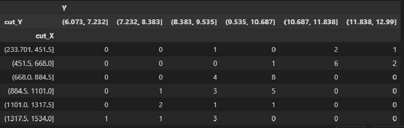

2. Let’s calculate the correlation ratio:

For further calculations, we reduce the correlation table to the type numpy.ndarray:

CorrTable_np = np.array(CorrTable_df)
print(CorrTable_np, type(CorrTable_np))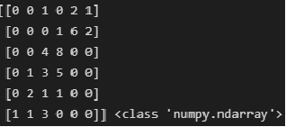

Results of the correlation table by rows and columns:

# итоги по строкам
n_group_X = [np.sum(CorrTable_np[i]) for i in range(K_X)]
print(f"n_group_X = {n_group_X}")

# итоги по столбцам
n_group_Y = [np.sum(CorrTable_np[:,j]) for j in range(K_Y)]
print(f"n_group_Y = {n_group_Y}")

We also need to get the group mean values X and Y for each group (interval). It should be remembered that the function pandas.crosstab when grouped, expands the extreme ranges by 0.1% on each side to include the minimum and maximum values.

To access data – interval boundaries obtained using pandas.cut – there are methods right and left:

# Среднегрупповые значения переменной X
Xboun_mean = [(CorrTable_df.index[i].left + CorrTable_df.index[i].right)/2 for i in range(K_X)]
Xboun_mean[0] = (np.min(X) + CorrTable_df.index[0].right)/2    # исправляем значения в крайних интервалах
Xboun_mean[K_X-1] = (CorrTable_df.index[K_X-1].left + np.max(X))/2
print(f"Xboun_mean = {Xboun_mean}")

# Среднегрупповые значения переменной Y
Yboun_mean = [(CorrTable_df.columns[j].left + CorrTable_df.columns[j].right)/2 for j in range(K_Y)]
Yboun_mean[0] = (np.min(Y) + CorrTable_df.columns[0].right)/2    # исправляем значения в крайних интервалах
Yboun_mean[K_Y-1] = (CorrTable_df.columns[K_Y-1].left + np.max(Y))/2
print(f"Yboun_mean = {Yboun_mean}", '\n')

Finding weighted averages X and Y for each group:

Xmean_group = [np.sum(CorrTable_np[:,j] * Xboun_mean) / n_group_Y[j] for j in range(K_Y)]
print(f"Xmean_group = {Xmean_group}")

Ymean_group = [np.sum(CorrTable_np[i] * Yboun_mean) / n_group_X[i] for i in range(K_X)]
print(f"Ymean_group = {Ymean_group}")

Total variance X and Y:

Sum2_total_X = np.sum(n_group_X * (Xboun_mean - np.mean(X))**2)
print(f"Sum2_total_X = {Sum2_total_X}")

Sum2_total_Y = np.sum(n_group_Y * (Yboun_mean - np.mean(Y))**2)
print(f"Sum2_total_Y = {Sum2_total_Y}")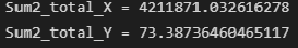

Intergroup variance X and Y (dispersion of group means):

Sum2_between_group_X = np.sum(n_group_Y * (Xmean_group - np.mean(X))**2)
print(f"Sum2_between_group_X = {Sum2_between_group_X}")

Sum2_between_group_Y = np.sum(n_group_X * (Ymean_group - np.mean(Y))**2)
print(f"Sum2_between_group_Y = {Sum2_between_group_Y}")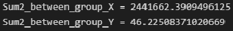

Intragroup variance X and Y (arises due to other factors – not related to another variable):

print(f"Sum2_within_group_X = {Sum2_total_X - Sum2_between_group_X}")
print(f"Sum2_within_group_Y = {Sum2_total_Y - Sum2_between_group_Y}")

Empirical correlation ratio:

corr_ratio_XY = sqrt(Sum2_between_group_Y / Sum2_total_Y)
print(f"corr_ratio_XY = {corr_ratio_XY}")

corr_ratio_YX = sqrt(Sum2_between_group_X / Sum2_total_X)
print(f"corr_ratio_YX = {corr_ratio_YX}")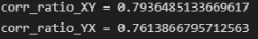

So, we got the result – the value of the correlation relation.

Let us estimate the tightness of the correlation Chaddock scalefor convenience, let’s create a custom function:

def Cheddock_scale_check(r, name="r"):
    # задаем шкалу Чеддока
    Cheddock_scale = {
        f'no correlation (|{name}| <= 0.1)':    0.1,
        f'very weak (0.1 < |{name}| <= 0.2)':   0.2,
        f'weak (0.2 < |{name}| <= 0.3)':        0.3,
        f'moderate (0.3 < |{name}| <= 0.5)':    0.5,
        f'perceptible (0.5 < |{name}| <= 0.7)': 0.7,
        f'high (0.7 < |{name}| <= 0.9)':        0.9,
        f'very high (0.9 < |{name}| <= 0.99)':  0.99,
        f'functional (|{name}| > 0.99)':        1.0}
    
    r_scale = list(Cheddock_scale.values())
    for i, elem in enumerate(r_scale):
        if abs(r) <= elem:
            conclusion_Cheddock_scale = list(Cheddock_scale.keys())[i]
            break
    return conclusion_Cheddock_scale

The Chaddock scale was originally intended to assess the tightness of a linear correlation relationship (based on the Pearson correlation coefficient r), but we will also apply it to the correlation relation η (not forgetting the property η ≥ r!). In function output cheddock_scale_check you can specify a symbol denoting a value – an argument name=chr(951) displays η instead of r.

In modern research Chaddock scale losing popularity, in recent years it has been increasingly used Evans scale (in psychosocial, biomedical, and other studies) (for more details about the scales of Chaddock, Evans, etc. – see.[4]). Let us estimate the tightness of the correlation Evans scalefor convenience, we will also create a custom function:

def Evans_scale_check(r, name="r"):
    # задаем шкалу Эванса
    Evans_scale = {
        f'very weak (|{name}| < 0.19)':         0.2,
        f'weak (0.2 < |{name}| <= 0.39)':       0.4,  
        f'moderate (0.4 < |{name}| <= 0.59)':   0.6,
        f'strong (0.6 < |{name}| <= 0.79)':     0.8,
        f'very strong (0.8 < |{name}| <= 1.0)': 1.0}
    
    r_scale = list(Evans_scale.values())
    for i, elem in enumerate(r_scale):
        if abs(r) <= elem:
            conclusion_Evans_scale = list(Evans_scale.keys())[i]
            break
    return conclusion_Evans_scale    

print(f"Оценка тесноты корреляции по шкале Эванса: {Evans_scale_check(corr_ratio_XY, name=chr(951))}")

So, the degree of correlation tightness can be estimated as high (according to the Chaddock scale), strong (according to the Evans scale).

3. Checking the significance of the correlation relationship:

Consider the null hypothesis:

H0: ηXY = 0
H1: ηXY ≠ 0

To test the null hypothesis, we use the Fisher criterion:

# расчетное значение статистики критерия Фишера
F_corr_ratio_calc = (n_X - K_X)/(K_X - 1) * corr_ratio_XY**2 / (1 - corr_ratio_XY**2)
print(f"Расчетное значение статистики критерия Фишера: F_calc = {round(F_corr_ratio_calc, DecPlace)}")
# табличное значение статистики критерия Фишера
dfn = K_X - 1
dfd = n_X - K_X
F_corr_ratio_table = sci.stats.f.ppf(p_level, dfn, dfd, loc=0, scale=1)
print(f"Табличное значение статистики критерия Фишера: F_table = {round(F_corr_ratio_table, DecPlace)}")
# расчетный уровень значимости
a_corr_ratio_calc = 1 - sci.stats.f.cdf(F_corr_ratio_calc, dfn, dfd, loc=0, scale=1)
print(f"Расчетный уровень значимости: a_calc = {round(a_corr_ratio_calc, DecPlace)}")
print(f"Заданный уровень значимости: a_level = {round(a_level, DecPlace)}")
# вывод
if F_corr_ratio_calc < F_corr_ratio_table:
    conclusion_corr_ratio_sign = f"Так как F_calc = {round(F_corr_ratio_calc, DecPlace)} < F_table = {round(F_corr_ratio_table, DecPlace)}" + \
        ", то гипотеза о равенстве нулю корреляционного отношения ПРИНИМАЕТСЯ, т.е. корреляционная связь НЕЗНАЧИМА"
else:
    conclusion_corr_ratio_sign = f"Так как F_calc = {round(F_corr_ratio_calc, DecPlace)} >= F_table = {round(F_corr_ratio_table, DecPlace)}" + \
        ", то гипотеза о равенстве нулю корреляционного отношения ОТВЕРГАЕТСЯ, т.е. корреляционная связь ЗНАЧИМА"
print(conclusion_corr_ratio_sign)

4. Confidence interval for the correlation ratio:

# число степеней свободы
f1 = round ((K_X - 1 + n_X * corr_ratio_XY**2)**2 / (K_X - 1 + 2 * n_X * corr_ratio_XY**2))
f2 = n_X - K_X
# вспомогательные величины
z1 = (n_X - K_X) / n_X * corr_ratio_XY**2 / (1 - corr_ratio_XY**2) * 1/sci.stats.f.ppf(p_level, f1, f2, loc=0, scale=1) - (K_X - 1)/n_X
z2 = (n_X - K_X) / n_X * corr_ratio_XY**2 / (1 - corr_ratio_XY**2) * 1/sci.stats.f.ppf(1 - p_level, f1, f2, loc=0, scale=1) - (K_X - 1)/n_X
# доверительный интервал
corr_ratio_XY_low = sqrt(z1) if sqrt(z1) >= 0 else 0
corr_ratio_XY_high = sqrt(z2) if sqrt(z2) <= 1 else 1
print(f"{p_level*100}%-ный доверительный интервал для корреляционного отношения: {[round(corr_ratio_XY_low, DecPlace), round(corr_ratio_XY_high, DecPlace)]}")

Important note: at values η close to 0 or 1 the left or right border of the confidence interval may go beyond the segment [0; 1]losing meaningful meaning (cm. [1, с.80]). The reason for this is in the approximation approach to determining the boundaries of the confidence interval. These adverse events are possible and should be taken into account when performing the analysis.

5. Checking the significance of the difference between a linear correlation and a non-linear one:

Let us estimate the value of the linear correlation coefficient:

corr_coef = sci.stats.pearsonr(X, Y)[0]
print(f"Коэффициент линейной корреляции: r = {round(corr_coef, DecPlace)}")

print(f"Оценка тесноты линейной корреляции по шкале Чеддока: {Cheddock_scale_check(corr_coef)}")
print(f"Оценка тесноты линейной корреляции по шкале Эванса: {Evans_scale_check(corr_coef)}")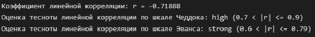

Let’s check the significance of the linear correlation coefficient:

# расчетный уровень значимости
a_corr_coef_calc = sci.stats.pearsonr(X, Y)[1]
print(f"Расчетный уровень значимости коэффициента линейной корреляции: a_calc = {a_corr_coef_calc}")
print(f"Заданный уровень значимости: a_level = {round(a_level, DecPlace)}")
# вывод
if a_corr_coef_calc >= a_level:
    conclusion_corr_coef_sign = f"Так как a_calc = {a_corr_coef_calc} >= a_level = {round(a_level, DecPlace)}" + \
        ", то гипотеза о равенстве нулю коэффициента линейной корреляции ПРИНИМАЕТСЯ, т.е. линейная корреляционная связь НЕЗНАЧИМА"
else:
    conclusion_corr_coef_sign = f"Так как a_calc = {a_corr_coef_calc} < a_level = {round(a_level, DecPlace)}" + \
        ", то гипотеза о равенстве нулю коэффициента линейной корреляции ОТВЕРГАЕТСЯ, т.е. линейная корреляционная связь ЗНАЧИМА"
print(conclusion_corr_coef_sign)

Now let’s check the significance of the difference between a linear correlation and a non-linear one. To do this, consider the null hypothesis:

H0: η² - r² = 0
H1: η² - r² ≠ 0

To test the null hypothesis, we use the Fisher criterion:

print(f"Корреляционное отношение: {chr(951)} = {round(corr_ratio_XY, DecPlace)}")
print(f"Коэффициент линейной корреляции: r = {round(corr_coef, DecPlace)}")
# расчетное значение статистики критерия Фишера
F_line_corr_sign_calc = (n_X - K_X)/(K_X - 2) * (corr_ratio_XY**2 - corr_coef**2) / (1 - corr_ratio_XY**2)
print(f"Расчетное значение статистики критерия Фишера: F_calc = {round(F_line_corr_sign_calc, DecPlace)}")
# табличное значение статистики критерия Фишера
dfn = K_X - 2
dfd = n_X - K_X
F_line_corr_sign_table = sci.stats.f.ppf(p_level, dfn, dfd, loc=0, scale=1)
print(f"Табличное значение статистики критерия Фишера: F_table = {round(F_line_corr_sign_table, DecPlace)}")
# расчетный уровень значимости
a_line_corr_sign_calc = 1 - sci.stats.f.cdf(F_line_corr_sign_calc, dfn, dfd, loc=0, scale=1)
print(f"Расчетный уровень значимости: a_calc = {round(a_line_corr_sign_calc, DecPlace)}")
print(f"Заданный уровень значимости: a_level = {round(a_level, DecPlace)}")
# вывод
if F_line_corr_sign_calc < F_line_corr_sign_table:
    conclusion_line_corr_sign = f"Так как F_calc = {round(F_line_corr_sign_calc, DecPlace)} < F_table = {round(F_line_corr_sign_table, DecPlace)}" + \
        f", то гипотеза о равенстве {chr(951)} и r ПРИНИМАЕТСЯ, т.е. корреляционная связь ЛИНЕЙНАЯ"
else:
    conclusion_line_corr_sign = f"Так как F_calc = {round(F_line_corr_sign_calc, DecPlace)} >= F_table = {round(F_line_corr_sign_table, DecPlace)}" + \
        f", то гипотеза о равенстве {chr(951)} и r ОТВЕРГАЕТСЯ, т.е. корреляционная связь НЕЛИНЕЙНАЯ"
print(conclusion_line_corr_sign)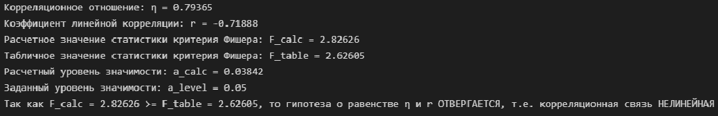

Creating a Custom Function for Correlation Analysis

For practical work, it is advisable to implement all the above calculations in the form of user-defined functions:

function corr_coef_check – to calculate and analyze Pearson’s linear correlation coefficient
function corr_ratio_check – to calculate and analyze the correlation relationship
function line_corr_sign_check – to check the significance of a linear correlation

These functions display the analysis results in the form of a DataFrame, which is convenient for visual perception and further use of the analysis results (however, the output method is at the discretion of each researcher).

# Функция для расчета и анализа коэффициента линейной корреляции Пирсона
def corr_coef_check(X, Y, p_level=0.95, scale="Cheddok"):
    a_level = 1 - p_level
    X = np.array(X)
    Y = np.array(Y)
    n_X = len(X)
    n_Y = len(Y)
    # оценка коэффициента линейной корреляции средствами scipy
    corr_coef, a_corr_coef_calc = sci.stats.pearsonr(X, Y)
    # несмещенная оценка коэффициента линейной корреляции (при n < 15) (см.Кобзарь, с.607)
    if n_X < 15:
        corr_coef = corr_coef * (1 + (1 - corr_coef**2) / (2*(n_X-3)))
    # проверка гипотезы о значимости коэффициента корреляции
    t_corr_coef_calc = abs(corr_coef) * sqrt(n_X-2) / sqrt(1 - corr_coef**2)
    t_corr_coef_table = sci.stats.t.ppf((1 + p_level)/2 , n_X - 2)
    conclusion_corr_coef_sign = 'significance' if t_corr_coef_calc >= t_corr_coef_table else 'not significance'
    # доверительный интервал коэффициента корреляции
    if t_corr_coef_calc >= t_corr_coef_table:
        z1 = np.arctanh(corr_coef) - sci.stats.norm.ppf((1 + p_level)/2, 0, 1) / sqrt(n_X-3) - corr_coef / (2*(n_X-1))
        z2 = np.arctanh(corr_coef) + sci.stats.norm.ppf((1 + p_level)/2, 0, 1) / sqrt(n_X-3) - corr_coef / (2*(n_X-1))
        corr_coef_conf_int_low = tanh(z1)
        corr_coef_conf_int_high = tanh(z2)
    else:
        corr_coef_conf_int_low = corr_coef_conf_int_high="-"    
    # оценка тесноты связи
    if scale=='Cheddok':
        conclusion_corr_coef_scale = scale + ': ' + Cheddock_scale_check(corr_coef)
    elif scale=='Evans':
        conclusion_corr_coef_scale = scale + ': ' + Evans_scale_check(corr_coef)
    # формируем результат            
    result = pd.DataFrame({
        'notation': ('r'),
        'coef_value': (corr_coef),
        'coef_value_squared': (corr_coef**2),
        'p_level': (p_level),
        'a_level': (a_level),
        't_calc': (t_corr_coef_calc),
        't_table': (t_corr_coef_table),
        't_calc >= t_table': (t_corr_coef_calc >= t_corr_coef_table),
        'a_calc': (a_corr_coef_calc),
        'a_calc <= a_level': (a_corr_coef_calc <= a_level),
        'significance_check': (conclusion_corr_coef_sign),
        'conf_int_low': (corr_coef_conf_int_low),
        'conf_int_high': (corr_coef_conf_int_high),
        'scale': (conclusion_corr_coef_scale)
        },
        index=['Correlation coef.'])
        
    return result

# Функция для расчета и анализа корреляционного отношения
def corr_ratio_check(X, Y, p_level=0.95, orientation='XY', scale="Cheddok"):
    a_level = 1 - p_level
    X = np.array(X)
    Y = np.array(Y)
    n_X = len(X)
    n_Y = len(Y)    
    # запишем данные в DataFrame
    matrix_XY_df = pd.DataFrame({
        'X': X,
        'Y': Y})
    # число интервалов группировки
    group_int_number = lambda n: round (3.31*log(n_X, 10)+1) if round (3.31*log(n_X, 10)+1) >=2 else 2
    K_X = group_int_number(n_X)
    K_Y = group_int_number(n_Y)
    # группировка данных и формирование корреляционной таблицы
    cut_X = pd.cut(X, bins=K_X)
    cut_Y = pd.cut(Y, bins=K_Y)
    matrix_XY_df['cut_X'] = cut_X
    matrix_XY_df['cut_Y'] = cut_Y
    CorrTable_df = pd.crosstab(
        index=matrix_XY_df['cut_X'],
        columns=matrix_XY_df['cut_Y'],
        rownames=['cut_X'],
        colnames=['cut_Y'])
    CorrTable_np = np.array(CorrTable_df)
    # итоги корреляционной таблицы по строкам и столбцам
    n_group_X = [np.sum(CorrTable_np[i]) for i in range(K_X)]
    n_group_Y = [np.sum(CorrTable_np[:,j]) for j in range(K_Y)]
    # среднегрупповые значения переменной X
    Xboun_mean = [(CorrTable_df.index[i].left + CorrTable_df.index[i].right)/2 for i in range(K_X)]
    Xboun_mean[0] = (np.min(X) + CorrTable_df.index[0].right)/2    # исправляем значения в крайних интервалах
    Xboun_mean[K_X-1] = (CorrTable_df.index[K_X-1].left + np.max(X))/2
    # среднегрупповые значения переменной Y
    Yboun_mean = [(CorrTable_df.columns[j].left + CorrTable_df.columns[j].right)/2 for j in range(K_Y)]
    Yboun_mean[0] = (np.min(Y) + CorrTable_df.columns[0].right)/2    # исправляем значения в крайних интервалах
    Yboun_mean[K_Y-1] = (CorrTable_df.columns[K_Y-1].left + np.max(Y))/2
    # средневзевешенные значения X и Y для каждой группы
    Xmean_group = [np.sum(CorrTable_np[:,j] * Xboun_mean) / n_group_Y[j] for j in range(K_Y)]
    Ymean_group = [np.sum(CorrTable_np[i] * Yboun_mean) / n_group_X[i] for i in range(K_X)]
    # общая дисперсия X и Y
    Sum2_total_X = np.sum(n_group_X * (Xboun_mean - np.mean(X))**2)
    Sum2_total_Y = np.sum(n_group_Y * (Yboun_mean - np.mean(Y))**2)
    # межгрупповая дисперсия X и Y (дисперсия групповых средних)
    Sum2_between_group_X = np.sum(n_group_Y * (Xmean_group - np.mean(X))**2)
    Sum2_between_group_Y = np.sum(n_group_X * (Ymean_group - np.mean(Y))**2)
    # эмпирическое корреляционное отношение
    corr_ratio_XY = sqrt(Sum2_between_group_Y / Sum2_total_Y)
    corr_ratio_YX = sqrt(Sum2_between_group_X / Sum2_total_X)
    try:
        if orientation!='XY' and orientation!='YX':
            raise ValueError("Error! Incorrect orientation!")
        if orientation=='XY':
            corr_ratio = corr_ratio_XY
        elif orientation=='YX':
            corr_ratio = corr_ratio_YX
    except ValueError as err:
        print(err)
    # проверка гипотезы о значимости корреляционного отношения
    F_corr_ratio_calc = (n_X - K_X)/(K_X - 1) * corr_ratio**2 / (1 - corr_ratio**2)
    dfn = K_X - 1
    dfd = n_X - K_X
    F_corr_ratio_table = sci.stats.f.ppf(p_level, dfn, dfd, loc=0, scale=1)
    a_corr_ratio_calc = 1 - sci.stats.f.cdf(F_corr_ratio_calc, dfn, dfd, loc=0, scale=1)
    conclusion_corr_ratio_sign = 'significance' if F_corr_ratio_calc >= F_corr_ratio_table else 'not significance'
    # доверительный интервал корреляционного отношения
    if F_corr_ratio_calc >= F_corr_ratio_table:
        f1 = round ((K_X - 1 + n_X * corr_ratio**2)**2 / (K_X - 1 + 2 * n_X * corr_ratio**2))
        f2 = n_X - K_X
        z1 = (n_X - K_X) / n_X * corr_ratio**2 / (1 - corr_ratio**2) * 1/sci.stats.f.ppf(p_level, f1, f2, loc=0, scale=1) - (K_X - 1)/n_X
        z2 = (n_X - K_X) / n_X * corr_ratio**2 / (1 - corr_ratio**2) * 1/sci.stats.f.ppf(1 - p_level, f1, f2, loc=0, scale=1) - (K_X - 1)/n_X
        corr_ratio_conf_int_low = sqrt(z1) if sqrt(z1) >= 0 else 0
        corr_ratio_conf_int_high = sqrt(z2) if sqrt(z2) <= 1 else 1
    else:
        corr_ratio_conf_int_low = corr_ratio_conf_int_high="-"    
    # оценка тесноты связи
    if scale=='Cheddok':
        conclusion_corr_ratio_scale = scale + ': ' + Cheddock_scale_check(corr_ratio, name=chr(951))
    elif scale=='Evans':
        conclusion_corr_ratio_scale = scale + ': ' + Evans_scale_check(corr_ratio, name=chr(951))
    # формируем результат            
    result = pd.DataFrame({
        'notation': (chr(951)),
        'coef_value': (corr_ratio),
        'coef_value_squared': (corr_ratio**2),
        'p_level': (p_level),
        'a_level': (a_level),
        'F_calc': (F_corr_ratio_calc),
        'F_table': (F_corr_ratio_table),
        'F_calc >= F_table': (F_corr_ratio_calc >= F_corr_ratio_table),
        'a_calc': (a_corr_ratio_calc),
        'a_calc <= a_level': (a_corr_ratio_calc <= a_level),
        'significance_check': (conclusion_corr_ratio_sign),
        'conf_int_low': (corr_ratio_conf_int_low),
        'conf_int_high': (corr_ratio_conf_int_high),
        'scale': (conclusion_corr_ratio_scale)
        },
        index=['Correlation ratio'])
    
    return result

# Функция для проверка значимости линейной корреляционной связи
def line_corr_sign_check(X, Y, p_level=0.95, orientation='XY'):
    a_level = 1 - p_level
    X = np.array(X)
    Y = np.array(Y)
    n_X = len(X)
    n_Y = len(Y)    
    # коэффициент корреляции
    corr_coef = sci.stats.pearsonr(X, Y)[0]
    # корреляционное отношение
    try:
        if orientation!='XY' and orientation!='YX':
            raise ValueError("Error! Incorrect orientation!")
        if orientation=='XY':
            corr_ratio = corr_ratio_check(X, Y, orientation='XY', scale="Evans")['coef_value'].values[0]
        elif orientation=='YX':
            corr_ratio = corr_ratio_check(X, Y, orientation='YX', scale="Evans")['coef_value'].values[0]
    except ValueError as err:
        print(err)
    # число интервалов группировки
    group_int_number = lambda n: round (3.31*log(n_X, 10)+1) if round (3.31*log(n_X, 10)+1) >=2 else 2
    K_X = group_int_number(n_X)
    # проверка гипотезы о значимости линейной корреляционной связи
    if corr_ratio >= abs(corr_coef):
        F_line_corr_sign_calc = (n_X - K_X)/(K_X - 2) * (corr_ratio**2 - corr_coef**2) / (1 - corr_ratio**2)
        dfn = K_X - 2
        dfd = n_X - K_X
        F_line_corr_sign_table = sci.stats.f.ppf(p_level, dfn, dfd, loc=0, scale=1)
        comparison_F_calc_table = F_line_corr_sign_calc >= F_line_corr_sign_table
        a_line_corr_sign_calc = 1 - sci.stats.f.cdf(F_line_corr_sign_calc, dfn, dfd, loc=0, scale=1)
        comparison_a_calc_a_level = a_line_corr_sign_calc <= a_level
        conclusion_null_hypothesis_check = 'accepted' if F_line_corr_sign_calc < F_line_corr_sign_table else 'unaccepted'
        conclusion_line_corr_sign = 'linear' if conclusion_null_hypothesis_check == 'accepted' else 'non linear'
    else:
        F_line_corr_sign_calc=""
        F_line_corr_sign_table=""
        comparison_F_calc_table=""
        a_line_corr_sign_calc=""
        comparison_a_calc_a_level=""
        conclusion_null_hypothesis_check = 'Attention! The correlation ratio is less than the correlation coefficient'
        conclusion_line_corr_sign = '-'
    
    # формируем результат            
    result = pd.DataFrame({
        'corr.coef.': (corr_coef),
        'corr.ratio.': (corr_ratio),
        'null hypothesis': ('r\u00b2 = ' + chr(951) + '\u00b2'),
        'p_level': (p_level),
        'a_level': (a_level),
        'F_calc': (F_line_corr_sign_calc),
        'F_table': (F_line_corr_sign_table),
        'F_calc >= F_table': (comparison_F_calc_table),
        'a_calc': (a_line_corr_sign_calc),
        'a_calc <= a_level': (comparison_a_calc_a_level),
        'null_hypothesis_check': (conclusion_null_hypothesis_check),
        'significance_line_corr_check': (conclusion_line_corr_sign),
        },
        index=['Significance of linear correlation'])
    
    return result

display(corr_coef_check(X, Y, scale="Evans"))
display(corr_ratio_check(X, Y, orientation='XY', scale="Evans"))
display(line_corr_sign_check(X, Y, orientation='XY'))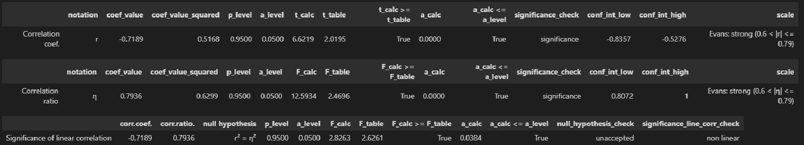

Let’s draw conclusions from the calculation results:

Between the quantities there is a significant (a_calc<0.05) correlation, correlation ratio η = 0.7936 (i.e. connection strong according to Evans).
The linear correlation between the quantities is also significant (a_calc<0.05), negative, correlation coefficient r = -0.7189 (connection strong according to Evans); linear correlation between variables explains 51.68% of the variation.
The hypothesis about the equality of the correlation ratio and the correlation coefficient is rejected (a_calc<0.05), that is, the difference between the linear form of the connection and the non-linear one is significant.

RESULTS

So, we have considered methods for constructing a correlation table, calculating the correlation ratio, checking its significance and constructing confidence intervals for it by means of Python. User-defined functions that reduce the size of the code are also proposed.

The source code is in my GitHub repository (https://github.com/AANazarov/Statistical-methods).

LITERATURE

Ayvazyan S.A. Applied Statistics: A Study of Dependencies. – M.: Finance and statistics, 1985. – 487 p.
Ayvazyan S.A., Mkhitaryan V.S. Applied statistics. Fundamentals of econometrics: In 2 volumes – V.1: Probability theory and applied statistics. – M.: UNITI-DANA, 2001. – 656 p.
Kobzar A.I. Applied mathematical statistics. For engineers and scientists. – M.: FIZMATLIT, 2006. – 816 p.
Koterov A.N. etc. The strength of communication. Message 2. Gradations of the magnitude of the correlation. – Medical radiology and radiation safety. 2019. Volume 64. No. 6. pp. 12–24 (https://medradiol.fmbafmbc.ru/journal_medradiol/abstracts/2019/6/12-24_Koterov_et_al.pdf).