Animating the wavefunction of a Schrödinger particle (ψ) with Python (with full code)

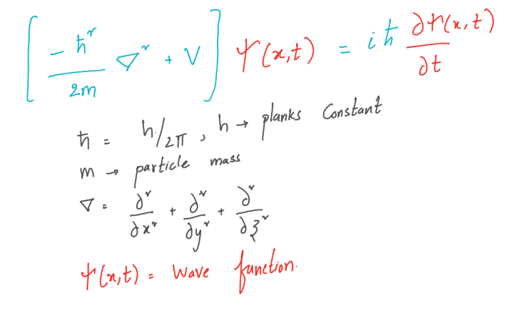
The dual nature of matter is a well-known concept among physicists. At the atomic level, matter behaves in some cases like particles and in others like waves. To explain this, we introduce the particle wave function ψ (x, t), which describes not the actual position of the particle, but the probability of finding the particle at a given point. The wave function ψ (x, t), or the probability field that satisfies perhaps the most important partial differential equation, at least for physicists, is the Schrödinger equation.

One-dimensional Schrödinger equation

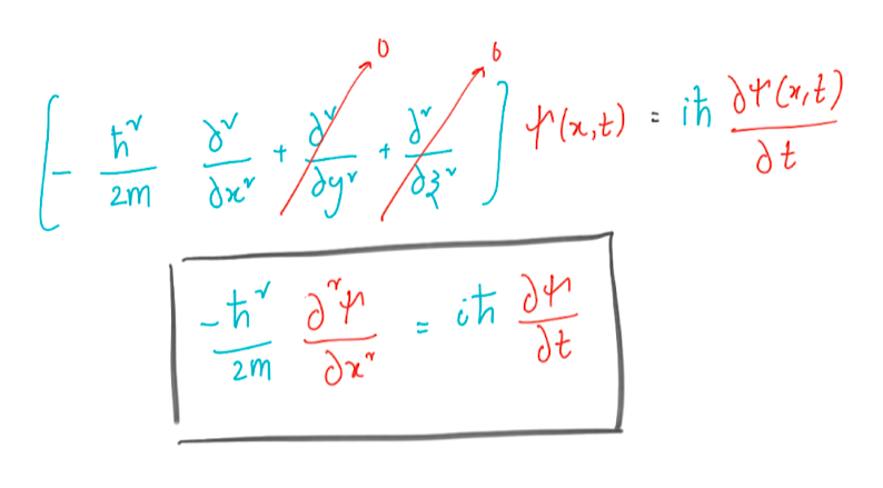
We will look at the Schrödinger equation in one dimension. The method for solving a wave function in two or three dimensions is basically the same as for one-dimensional. But for visualization and for the sake of saving time, we will stick to one dimension. Let us derive the Schrödinger equation for the one-dimensional case.

Solving a particle in a box by the Crank – Nicholson method

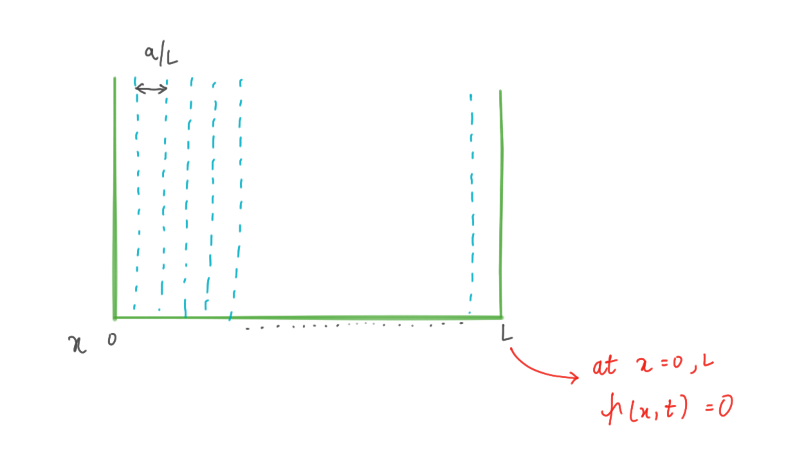
Let’s solve the wave equation for our particle in a box with impenetrable walls. The idea is to solve the equation in a finite space. But why in impenetrable walls? This condition makes the wave function equal to zero on the walls, which we put at x = 0 and x = L. We replace the second derivative in the Schrödinger equation with a finite difference and apply Euler’s method.

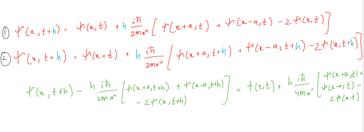
The above derivation allows us to recursively solve the Schrödinger equation. Boundary conditions at x = 0 and x = L for all t, the wave function ψ (x, t) = 0. Between these points, we have grid points at points a, 2a, 3a, and so on. Let us group the values ψ (x, t) at these interior points into a vector.

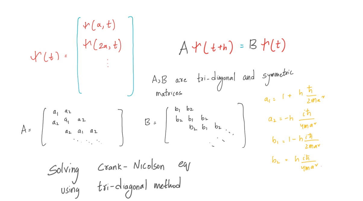
Now everything is simple, we have a propagation function: Aψ (t + h) = Bψ
from pylab import *
from matplotlib import pyplot as plt
from matplotlib import animation
#matplotlib.use(‘GTK3Agg’)

# from matplotlib import interactive
# interactive(True)

########################################Variables######################################################################################################
N_Slices = 1000 #Number of slices in the box
Time_step = 1e-18 #Time step for each iteration
Mass = 9.109e-31 #mass of electron
plank = 1.0546e-36 #Planks constant
L_Box = 1e-9 #Length of the box
Grid = L_Box/N_Slices #Lenght of each slice

#####################################Si(0) using the given equation ###############################################################################

Si_0 = np.zeros(N_Slices+1,complex) #Initiating Si funtion at time step = 0
x = np.linspace(0,L_Box,N_Slices+1)
def G_Equation(x):
x_0 = L_Box/2
Sig = 1e-10
k = 5e10
result = exp(-(x-x_0)**2/2/Sig**2)*exp(1j*k*x) #Given Equation at t = 0
return result
Si_0[:] = G_Equation(x) #Si funtion at time step = 0

#######################################V = Bxsi(0)################################################################################
a_1 = 1 + Time_step*plank*1j/(2*Mass*(Grid**2)) #Diagonal of A Tridiagonal matrix
a_2 = -Time_step*plank*1j/(4*Mass*Grid**2) #Up and Down to A Tridiagonal matrix
b_1 = 1 – Time_step*plank*1j/(2*Mass*(Grid**2)) #Diagonal of B Tridiagonal matrix
b_2 = Time_step*plank*1j/(4*Mass*Grid**2) #Up and Down to B Tridiagonal matrix

BxSi_0 = [] #V = BxSi and si funtion at x = 0
for i in range(1000):
if i == 0:
BxSi_0.append(b_1*Si_0[0] + b_2*(Si_0[1])) #V can be maipulated by the equation in Text book
else:
BxSi_0.append(b_1*Si_0[i] + b_2*(Si_0[i+1] + Si_0[i-1]))
BxSi_0 = np.array(BxSi_0)

#####################################Tri Diagonal matrix algorithm#####################################################################################

def TDMAsolver(a, b, c, d): #Instead of solving using Numpy.linalg, it is prefered to Use
nf = len(d) #Tri Diagonal Matrix algorithm
ac, bc, cc, dc = map(np.array, (a, b, c, d)) # a,b,c’s are up,dia,down element in tridiagonl matrix A
for it in range(1, nf): #AX = d
mc = ac[it-1]/bc[it-1]
bc[it] = bc[it] – mc*cc[it-1]
dc[it] = dc[it] – mc*dc[it-1]

xc = bc
xc[-1] = dc[-1]/bc[-1]

for il in range(nf-2, -1, -1):
xc[il] = (dc[il]-cc[il]*xc[il+1])/bc[il]
return xc

global a #A matrix is fixed through out the problem, so it is good to globalize the variables
global b
global c
b = N_Slices*[a_1] #In A matrix, Both Up,Down elements are a_2 and diag matrix is a_1
a = (N_Slices-1)*[a_2]
c = (N_Slices-1)*[a_2]
####################################Si 1st funtion solver####################################################################################

global Si_1 #First si_funtion usinf Axsi(0+h) = BxSi(0)
Si_1 = TDMAsolver(a, b, c, BxSi_0) #This can be solved by TDM(A,BxSi(0))

###################################A funtion which caliculates si at each step#####################################################################################
global Si_sd #AxSi_stepup = BxSi_stepdown
Si_sd = {} #At first Buckting Si_stepdown in to directry which we can using for finding Si_stepup
def sifuntion(i): #In next iteration, Last iteration Si_stepup will be this iteration’s Si_stepdown
if i == 0:
Si_sd[0] = Si_1
return Si_1
else:
Si_stepdown = Si_sd[i-1]
V = np.zeros(N_Slices,complex)
V[0] = b_1*Si_stepdown[0] + b_2*(Si_stepdown[1])
V[1:N_Slices-1] = b_1*Si_stepdown[1:N_Slices-1] + b_2*(Si_stepdown[2:N_Slices] + Si_stepdown[0:N_Slices-2])
V[N_Slices-1] = b_1*Si_stepdown[N_Slices-1]+ b_2*(Si_stepdown[N_Slices-2])
Si_stepup = TDMAsolver(a, b, c, V)
Si_sd[i] = Si_stepup
x = Si_stepup.real
return x
####################################Animating#######################################################################################

fig = plt.figure()
ax = plt.axes(xlim=(0, 1000), ylim=(-1.5, 1.5))
line, = ax.plot([], [], lw=5)
ax.legend(prop=dict(size=20))
ax.set_facecolor(‘black’)
ax.patch.set_alpha(0.8)
ax.set_xlabel(‘$x$’,fontsize = 15,color=”blue”)
ax.set_ylabel(r’$|psi(x)|$’,fontsize = 15,color=”blue”)
ax.grid(color=”blue”)
ax.set_title(r’$|psi(x)|$ vs $x$’, color=”blue”,fontsize = 15 )
line, = ax.step([], [])

def init():
line.set_data([], [])
return line,

def animate(i):
x = np.linspace(0, 1000, num=1000)
y = sifuntion(i)
line.set_data(x, y)
line.set_color(‘red’)
return line,

anim = animation.FuncAnimation(fig, animate, init_func=init,
frames=10**5, interval=1, blit=True)#5*10**5

plt.vlines(1, -5, 5, linestyles=”solid”, color=”green”,lw=5)
plt.vlines(999, -5, 5, linestyles=”solid”, color=”green”,lw=5)
plt.text(1,1,’Boundary’,rotation=90,color=”green” )
plt.text(975,1,’Boundary’,rotation=90,color=”green” )
plt.figure(figsize=(10,10))
plt.show()

# Writer = animation.writers[‘ffmpeg’]
# writer = Writer()
# anim.save(‘im.mp4’, writer=writer)